Part of my role at MathWorks involves supporting academics in the use of their tools. Every now and then I get involved with co-supervising projects which usually involves some element of assessment. Ever since the advent of ChatGPT, I have noticed that students like to ‘delve’ into topics a lot more than they used to. The topics that are being delved into often involve a ‘complex interplay’ of something or maybe there’s reference to an ‘intricate dance’ while the reader is invited to go on a ‘journey’.
I recently had the opportunity to appear on Jousef Murad’s podcast Deep Dive. My appearance was sponsored by my employer, MathWorks, but I was given free reign to talk about pretty much whatever I wanted. So I chose to talk about Research Software Engineering and the techniques from software engineering that I think every scientist and engineer should employ (e.g. Version Control!). MATLAB and MathWorks is mentioned a bit but the aim of the podcast was that it would be of interest to anyone who has to do technical computing in any programming language.
WalkingRandomly is coming up to its 15th Anniversary! When I started blogging in 2007, I never would have believed that this little corner of the web would still be going in 2022!
As you might have noticed, posting frequency has waned over recent years which is partly to do with Real Life taking over somewhat but also because my professional life has become rather more hectic over the years. When I started posting here, I was a junior research computing specialist and when I left academia in 2019 I was a head of Research Computing for a major UK University! It was a wild ride.
In 2019 I joined the commercial world with The Numerical Algorithms Group where I spent a lovely couple of years immersing myself in commercial cloud, HPC and numerical computing.
A new beginning
At the beginning of 2021, in the deepest depths of the pandemic, I was offered the opportunity to join MathWorks, The Makers of MATLAB, to work with academia as a ‘Customer Success Engineer’. Broadly speaking, I help researchers and educators solve their problems with MATLAB.
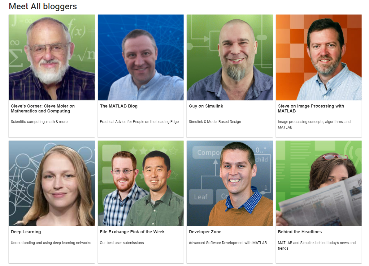
Things have been going pretty well and earlier this month they gave me my own blog on MathWorks Central. Little old me right next to the original developer of MATLAB, Cleve Moler, in the gallery of MathWorks bloggers.
The new blog is called simply The MATLAB blog but as you might expect from someone who has spent 15 years writing about many aspects of scientific computing, there’s going to be a lot more than just MATLAB on there. Expect to see posts on subjects such as HPC, Research Software Engineering, C++, Python, GPUs and maybe even a little Fortran!
www.walkingrandomly.com won’t be going away and I’ll still post here from time to time but, for the forseeable future at least, most of my output will be on The MATLAB blog.
It only took me 15 years but I finally figured out how to get paid for blogging :)
The MATLAB community site, MATLAB Central, is celebrating its 20th anniversary with a coding competition where the only aim is to make an interesting image with under 280 characters of code. The 280 character limit ensures that the resulting code is tweetable. There are a couple of things I really like about the format of this competition, other than the obvious fact that the only aim is to make something pretty!
No MATLAB license is required! Sign up for a free MathWorks account and away you go. You can edit and run code in the browser.
Stealing reusing other people’s code is actively encouraged! The competition calls it remixing but GitHub users will recognize it as forking.
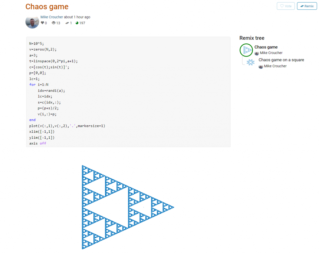
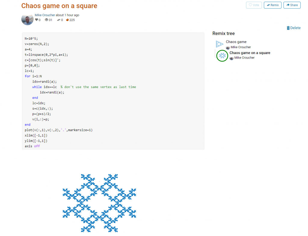
This is about as simple as the Chaos game gets and there are many things that could be done to produce a different image. As you can see from the Remix tree on the right hand side, I’ve already done one of them by changing a from 3 to 4 and adding some extra code to ensure that the same vertex doesn’t get chosen twice. This is result:
Someone else can now come along, hit the remix button and edit the code to produce something different again. Some things you might want to try for the chaos game include
Try changing the value of a which is used in the variables t and c to produce the vertices of a polygon on an enclosing circle.
Instead of just using the vertices of a polygon, try using the midpoints or another scheme for producing the attractor points completely.
Try changing the scaling factor — currently p=(p+s)/2;
Try putting limitations on which vertex is chosen. This remix ensures that the current vertex is different from the last one chosen.
Each vertex is currently equally likely to be chosen using the code idx=randi(a); Think of ways to change the probabilities.
Think of ways to colorize the plots.
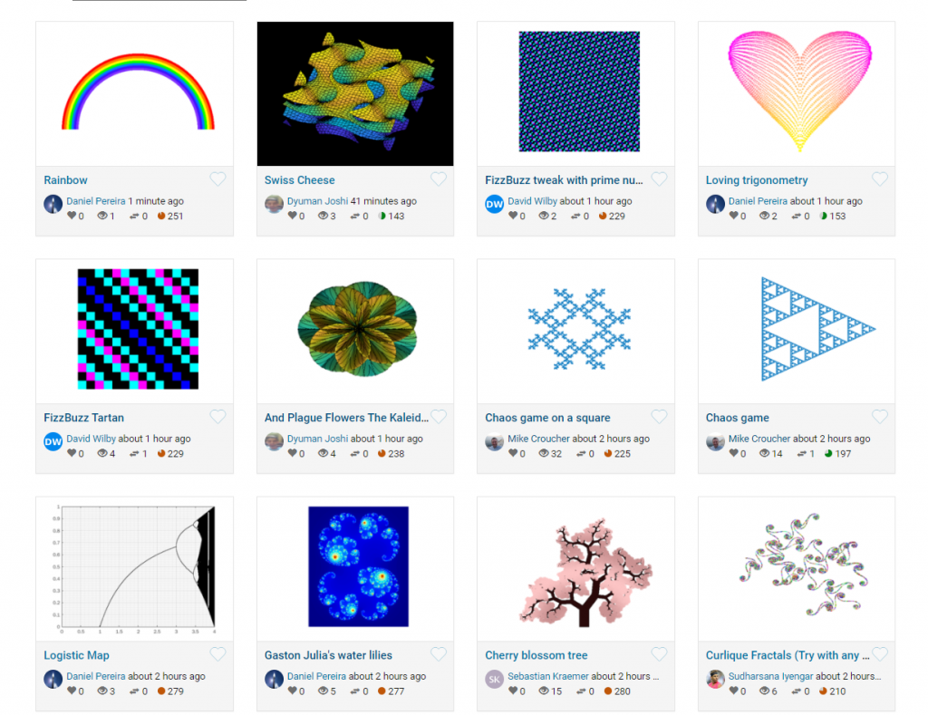
Maybe the chaos game isn’t your thing. You are free to create your own design from scratch or perhaps you’d prefer to remix some of the other designs in the gallery.
The competition is just a few hours old and there are already some very nice ideas coming out.
Fast forward to 2021 and my personal computational landscape has changed substantially. The pandemic has confined me to my home office and high performance laptops don’t have quite the same allure that they did when I was doing most of my interesting computational work in airports and coffee shops. I swapped a 15 inch screen for a 49 inch Ultrawide monitor and my laptop is gathering dust while I enjoy my new Dell desktop with an 8 core Intel i7-11700 and an NVIDIA GTX 3070.
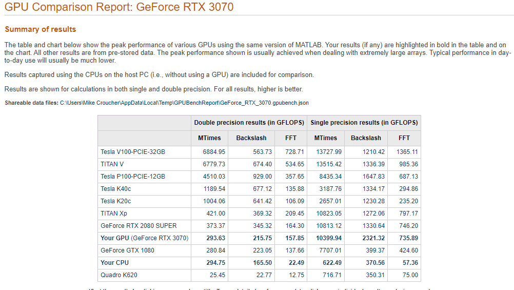
This is the first desktop machine I’ve personally owned for almost two decades and the amount of performance I got for less money than the high spec laptops I used to favour is astonishing! Here are the GPU Bench results using MATLAB 2021a
The standout figure is 10,399 Gigaflops for single precision Matrix-Matrix multiplication. At only slightly shy of 10.4 Teraflops that’s almost an order of magnitude faster than the results that impressed me on my laptop 4 years ago!
Double precision performance is nothing to write home about but it never is on consumer NVIDIA GPU cards. I stopped being upset about that years ago!
The other result I find interesting with respect to my personal history of devices is the 622 Gigaflops result for single precision from the Intel i7 CPU. This is getting on for twice as fast as the GPU on my 2015 Apple MacbookPro which managed 349 Gigaflops….a machine I still use today although primarily for Netflix.
Micro Visual Proofs – Animated proofs without words
Proofs without words have been around for a long time. Diagrams that demonstrate that a mathematical statement is ‘obviously’ true. The example that always springs to my mind is the one below that demonstrates that the sum of consecutive odd numbers is a square number.
Tom Edgar has been working on videos that animate proofs without words for a new YouTube channel called Micro Visual Proofs and submitted the one below for this month’s Carnival of math.
2.648102… Has anyone seen this constant?
Peter Cameron has been working on graphs on groups and has come across the constant 2.648102…. In this post he discusses how it turned up and asks if anyone else has come across it. There’s an interesting discussion in the comments section
Electrostatics and the Gauss–Lucas Theorem
Insight into mathematical theorems can come from many different places with physics being an extremely common one! Physical problems can be very useful in making even the most abstract concepts more concrete. John Carlos-Baez demonstrates this perfectly in his post Electrostatics and the Gauss-Lucas Theorem
Mathematics from TikTok
When the carnival of mathematics first began, it was all about mathematical blogs – a medium that was relatively new at the time. There was something wonderful about seeing mathematicians, scientists, teachers and hobbyists communicating more directly with the world. Internet time moves quickly and there has since been an explosion of interesting mathematical discussion on many other social media platforms — one of these being TikTok.
In this twitter post by Howie Hua, a teacher of math to future elementary school teachers, Howie advertises a TikTok video where he asks ‘What Happens if we add fractions across?’
“In this profile video of applied mathematician Bronwyn Hajek from the University of South Australia, Hajek describes how she is motivated by the
quest to solve tricky, obscure, unsolved partial differential equations. Hajek will visit the Sydney Mathematical Research Institute in coming
months to collaborate on a project to apply Lie symmetry methods to model biological shocks.
I hope you like this video, which covers her upcoming project and some of the mathematical breakthroughs that Hajek has been involved with in recent years.”
Chalkdust – A magazine for the mathematically curious
Robin Whitty submitted this post that celebrates the launch of issue 13 of the Chalkdust magazine which focuses on John Conway, creator of the game of life, among many other things.
Earlier this week Apple announced their new, Arm-based ‘Apple Silicon’ machines to the world in a slick marketing event that had many of us reaching for our credit cards. Simultaneously, The Numerical Algorithms Group announced that they had ported their Fortran Compiler to the new platform. At the time of writing this is the only Fortran compiler publicly available for Apple Silicon although that will likely change soon as open source Fortran compilers get updated.
At over 60 years old, Fortran is one of the oldest programming languages that continues to be actively developed and used (The latest language specification is Fortran 2018). Routinely mocked by software engineers as old-skool (including me who, over a decade ago, suggested that it shouldn’t be taught to undergraduates), Fortran is the language that everyone overlooks as they spend their days sipping flat-whites in Starbucks while hacking away in MATLAB, R or Python on shiny Macbook Airs.
It can come as quite a shock, therefore, to discover that much of our favourite data science tools simply cannot work natively on any system that doesn’t have a Fortran compiler!
It’s Fortran all the way down
Much of the numerical functionality we routinely use today was developed decades ago and released in Fortran. More modern systems, such as R, make direct use of a lot of this code because it is highly performant and, perhaps more importantly, has been battle tested in production for decades. Numerical computing is hard (even when all of your instincts suggest otherwise) and when someone demonstrably does it right, it makes good sense to reuse rather than reinvent.
As a result, with no Fortran, there’s no R.
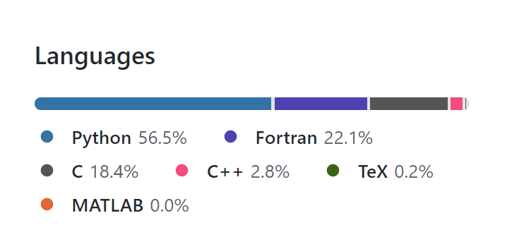
The Python crowd don’t get away with it either. Here are the GitHub stats for Scipy as of today
Of course, no Scipy means you also can’t have anything that depends on Scipy including things like Keras or Scikit-learn. Also, if you want good performance for linear algebra operations (Which underpins a huge number of data science and ML algorithms) then you’ll need a good BLAS implementation. Many projects use OpenBLAS (It’s a popular option in Numpy for example) which…you guessed it…is almost 49% Fortran.
Emulation for now
NAG’s Fortran compiler is excellent (it routinely tops independent charts for its checking and Fortran standards compliance for example) but it is commercial. The community needs and will demand open source (or at least free) Fortran compilers if data scientists are ever going to realise the full potential of Apple’s new hardware and I have no doubt that these are on the way. Other major silicon providers (e.g. Intel, AMD, NEC and NVIDIA/PGI) have their own Fortran compiler that co-exist with the open ones. Perhaps Apple should join the club (I suggest they talk to NAG!).
Until this is resolved, most of us will be relying on the Rosetta2 emulation…which, thankfully, is apparently pretty good!
At the time of writing, Microsoft Azure has 3 High Performance Computing instances available and I often find myself looking up their specifications and benchmark results when discussing their various methods with colleagues and clients. All the information is out there but seems to be spread across several documents. To save me the trouble in future, here is everything I usually need in one place
HC nodes: Original source of data
* CPU: Intel Skylake
* Cores: 44 (non-hyperthreaded)
* 3.5 TeraFLOPS double precision peak
* 352 Gigabyte RAM
* 700 Gigabyte local SSD storage
* 190 GB/s memory bandwidth
* 100 GB/s infiniband
HB Nodes: Original source of data
* CPU: AMD EPYC 7000 series (Naples)
* Cores: 60 (non-hyperthreaded)
* ???? Peak double precision peak
* 240 Gigabyte RAM
* 700 Gigabyte local SSD storage
* 263 GB/s memory bandwidth
* 100 GB/s infiniband
HBv2 nodes: Original source of data
* CPU: AMD EPYC 7002 series (Rome)
* Cores: 120 (non-hyperthreaded)
* 4 TeraFlops Peak double precision
* 480 Gigabyte RAM
* 1.6 Terabyte local SSD storage
* 350 GB/s memory bandwidth
* 200 GB/s infiniband
az group create --name <rg_name> --location <location>
Where you replace <location>with the region where you want to create the resource group. You may have a region in mind (South Central US perhaps) or you may be wondering which regions are available. Either way, it is helpful to see the list of all possible values for <location> in commands like the one above.
Let’s get the output in a more human readable table format.
az account list-locations -o table

DisplayName           Latitude    Longitude    Name
--------------------  ----------  -----------  ------------------
East Asia             22.267      114.188      eastasia
Southeast Asia        1.283       103.833      southeastasia
Central US            41.5908     -93.6208     centralus
East US               37.3719     -79.8164     eastus
East US 2             36.6681     -78.3889     eastus2
West US               37.783      -122.417     westus
North Central US      41.8819     -87.6278     northcentralus
South Central US      29.4167     -98.5        southcentralus
North Europe          53.3478     -6.2597      northeurope
West Europe           52.3667     4.9          westeurope
Japan West            34.6939     135.5022     japanwest
Japan East            35.68       139.77       japaneast
Brazil South          -23.55      -46.633      brazilsouth
Australia East        -33.86      151.2094     australiaeast
Australia Southeast   -37.8136    144.9631     australiasoutheast
South India           12.9822     80.1636      southindia
Central India         18.5822     73.9197      centralindia
West India            19.088      72.868       westindia
Canada Central        43.653      -79.383      canadacentral
Canada East           46.817      -71.217      canadaeast
UK South              50.941      -0.799       uksouth
UK West               53.427      -3.084       ukwest
West Central US       40.890      -110.234     westcentralus
West US 2             47.233      -119.852     westus2
Korea Central         37.5665     126.9780     koreacentral
Korea South           35.1796     129.0756     koreasouth
France Central        46.3772     2.3730       francecentral
France South          43.8345     2.1972       francesouth
Australia Central     -35.3075    149.1244     australiacentral
Australia Central 2   -35.3075    149.1244     australiacentral2
UAE Central           24.466667   54.366669    uaecentral
UAE North             25.266666   55.316666    uaenorth
South Africa North    -25.731340  28.218370    southafricanorth
South Africa West     -34.075691  18.843266    southafricawest
Switzerland North     47.451542   8.564572     switzerlandnorth
Switzerland West      46.204391   6.143158     switzerlandwest
Germany North         53.073635   8.806422     germanynorth
Germany West Central  50.110924   8.682127     germanywestcentral
Norway West           58.969975   5.733107     norwaywest
Norway East           59.913868   10.752245    norwayeast
The entries in the Name column are valid options for <location> in the command we started out with.
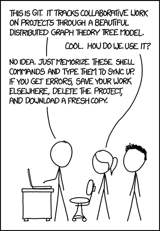
Many people suggest that you should use version control as part of your scientifc workflow. This is usually quickly followed up by recommendations to learn git and to put your project on GitHub. Learning and doing all of this for the first time takes a lot of effort. Alongside all of the recommendations to learn these technologies are horror stories telling how difficult it can be and memes saying that no one really knows what they are doing!
There are a lot of reasons to not embrace the git but there are even more to go ahead and do it. This is an attempt to convince you that it’s all going to be worth it alongside a bunch of resources that make it easy to get started and academic papers discussing the issues that version control can help resolve.
This document will not address how to do version control but will instead try to answer the questions what you can do with it and why you should bother. It was inspired by a conversation on twitter.
Improvements to individual workflow
Ways that git and GitHub can help your personal computational workflow – even if your project is just one or two files and you are the only person working on it.
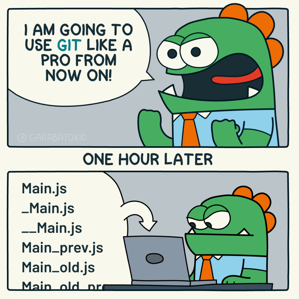
Fixing filename hell
Is this a familiar sight in your working directory?
For many people, this is just the beginning. For a project that has existed long enough there might be dozens or even hundreds of these simple scripts that somehow define all of part of your computational workflow. Version control isn’t being used because ‘The code is just a simple script developed by one person’ and yet this situation is already becoming the breeding ground for future problems.
Which one of these files is the most up to date?
Which one produced the results in your latest paper or report?
Which one contains the new work that will lead to your next paper?
Which ones contain deep flaws that should never be used as part of the research?
Which ones contain possibly useful ideas that have since been removed from the most recent version?
Applying version control to this situation would lead you to a folder containing just one file
mycode.py
All of the other versions will still be available via the commit history. Nothing is ever lost and you’ll be able to effectively go back in time to any version of mycode.py you like.
A single point of truth
I’ve even seen folders like the one above passed down generations of PhD students like some sort of family heirloom. I’ve seen labs where multple such folders exist across a dozen machines, each one with a mixture of duplicated and unique files. That is, not only is there a confusing mess of files in a folder but there is a confusing mess of these folders!
This can even be true when only one person is working on a project. Perhaps you have one version of your folder on your University HPC cluster, one on your home laptop and one on your work machine. Perhaps you email zipped versions to yourself from time to time. There are many everyday events that can lead to this state of affairs.
By using a GitHub repository you have a single point of truth for your project. The latest version is there. All old versions are there. All discussion about it is there.
Everything…one place.
The power of this simple idea cannot be overstated. Whenever you (or anyone else) wants to use or continue working on your project, it is always obvious where to go. Never again will you waste several days work only to realise that you weren’t working on the latest version.
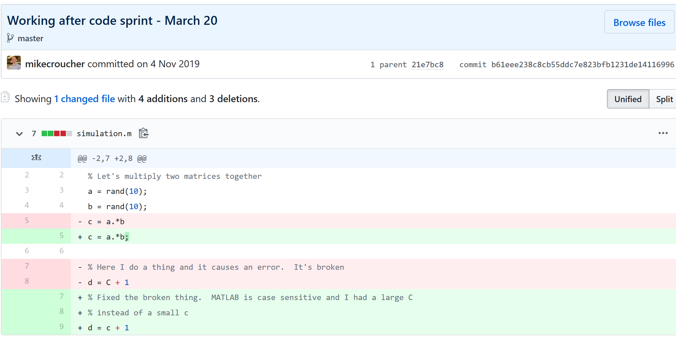
Keeping track of everything that changed
The latest version of your analysis or simulation is different from the previous one. Thanks to this, it may now give different results today compared to yesterday. Version control allows you to keep track of everything that changed between two versions. Every line of code you added, deleted or changed is highlighted. Combined with your commit messages where you explain why you made each set of changes, this forms a useful record of the evolution of your project.
It is possible to compare the differences between any two commits, not just two consecutive ones which allows you to track the evolution of your project over time.
Always having a working version of your project
Ever noticed how your collaborator turns up unnanounced just as you are in the middle of hacking on your code. They want you to show them your simulation running but right now its broken! You frantically try some of the other files in your folder but none of them seem to be the version that was working last week when you sent the report that moved your collaborator to come to see you.
If you were using version control you could easily stash your current work, revert to the last good commit and show off your work.
Tracking down what went wrong
You are always changing that script and you test it as much as you can but the fact is that the version from last year is giving correct results in some edge case while your current version is not. There are 100 versions between the two and there’s a lot of code in each version! When did this edge case start to go wrong?
With git you can use git bisect to help you track down which commit started causing the problem which is the first step towards fixing it.
Providing a back up of your project
Try this thought experiment: Your laptop/PC has gone! Fire, theft, dead hard disk or crazed panda attack.
It, and all of it’s contents have vanished forever. How do you feel? What’s running through your mind? If you feel the icy cold fingers of dread crawling up your spine as you realise Everything related to my PhD/project/life’s work is lost then you have made bad life choices. In particular, you made a terrible choice when you neglected to take back ups.
Of course there are many ways to back up a project but if you are using the standard version control workflow, your code is automatically backed up as a matter of course. You don’t have to remember to back things up, back-ups happen as a natural result of your everyday way of doing things.
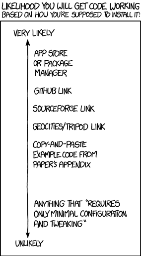
Making your project easier to find and install
There are dozens of ways to distribute your software to someone else. You could (HORRORS!) email the latest version to a colleuage or you could have a .zip file on your web site and so on.
Each of these methods has a small cognitive load for both recipient and sender. You need to make sure that you remember to update that .zip file on your website and your user needs to find it. I don’t want to talk about the email case, it makes me too sad. If you and your collaborator are emailing code to each other, please stop. Think of the children!
One great thing about using GitHub is that it is a standardised way of obtaining software. When someone asks for your code, you send them the URL of the repo. Assuming that the world is a better place and everyone knows how to use git, you don’t need to do anything else since the repo URL is all they need to get your code. a git clone later and they are in business.
Additionally, you don’t need to worry abut remembering to turn your working directory into a .zip file and uploading it to your website. The code is naturally available for download as part of the standard workflow. No extra thought needed!
In addition to this, some popular computational environments now allow you to install packages directly from GitHub. If, for example, you are following standard good practice for building an R package then a user can install it directly from your GitHub repo from within R using the devtools::install_github() function.
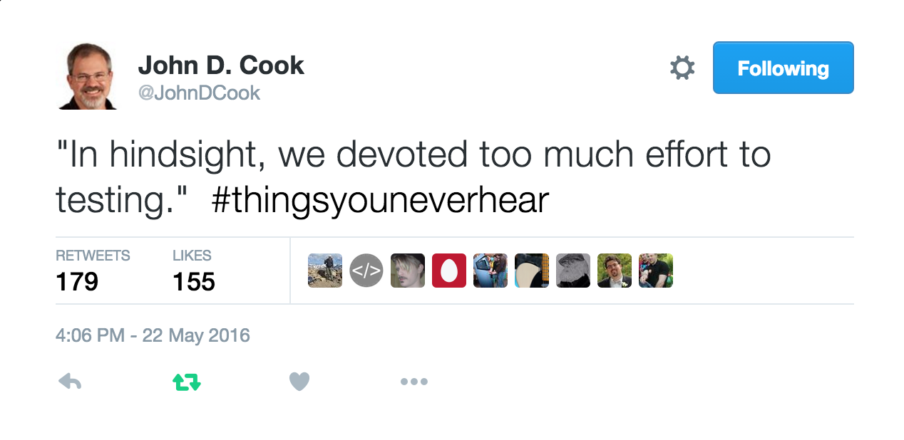
Automatically run all of your tests
You’ve sipped of the KoolAid and you’ve been writing unit tests like a pro. GitHub allows you to link your repo with something called Continuous Integration (CI) that helps maximise the utility of those tests.
Once its all set up the CI service runs every time you, or anyone else, makes a commit to your project. Every time the CI service runs, a virtual machine is created from scratch, your project is installed into it and all of your tests are run with any failures reported.
This gives you increased confidence that everything is OK with your latest version and you can choose to only accept commits that do not break your testing framework.
Collaboration and Community
How git and GitHub can make it easier to collaborate with others on computational projects.
Control exactly who can see your work
‘I don’t want to use GitHub because I want to keep my project private’ is a common reason given to me for not using the service. The ability to create private repositories has been free for some time now (Price plans are available here https://github.com/pricing) and you can have up to 3 collaborators on any of your private repos before you need to start paying. This is probably enough for most small academic projects.
This means that you can control exactly who sees your code. In the early stages it can be just you. At some point you let a couple of trusted collaborators in and when the time is right you can make the repo public so everyone can enjoy and use your work alongside the paper(s) it supports.
Faciliate discussion about your work
Every GitHub repo comes with an Issues section which is effectively a discussion forum for the project. You can use it to keep track of your project To-Do list, bugs, documentation discussions and so on. The issues log can also be integrated with your commit history. This allows you to do things like git commit -m "Improve the foo algorithm according to the discussion in #34" where #34 refers to the Issue discussion where your collaborator pointed out
Allow others to contribute to your work
You have absolute control over external contributions! No one can make any modifications to your project without your explicit say-so.
I start with the above statement because I’ve found that when explaining how easy it is to collaborate on GitHub, the first question is almost always ‘How do I keep control of all of this?’
What happens is that anyone can ‘fork’ your project into their account. That is, they have an independent copy of your work that is clearly linked back to your original. They can happily work away on their copy as much as they like – with no involvement from you. If and when they want to suggest that some of their modifications should go into your original version, they make a ‘Pull Request’.
I emphasised the word ‘Request’ because that’s exactly what it is. You can completely ignore it if you want and your project will remain unchanged. Alternatively you might choose to discuss it with the contributor and make modifications of your own before accepting it. At the other end of the spectrum you might simply say ‘looks cool’ and accept it immediately.
Congratulations, you’ve just found a contributing collaborator.
Reproducible research
How git and GitHub can contribute to improved reproducible research.
Simply making your software available
A paper published without the supporting software and data is (much!) harder to reproduce than one that has both.
Making your software citable
Most modern research cannot be done without some software element. Even if all you did was run a simple statistical test on 20 small samples, your paper has a data and software dependency. Organisations such as the Software Sustainability Institute and the UK Research Software Engineering Association (among many others) have been arguing for many years that such software and data dependencies should be part of the scholarly record alongside the papers that discuss them. That is, they should be archived and referenced with a permanent Digital Object Identifier (DOI).
Once your code is in GitHub, it is straightforward to archive the version that goes with your latest paper and get it its own DOI using services such as Zenodo. Your University may also have its own archival system. For example, The University of Sheffield in the UK has built a system called ORDA which is based on an institutional Figshare instance which allows Sheffield academics to deposit code and data for long term archival.
Which version gave these results?
Anyone who has worked with software long enough knows that simply stating the name of the software you used is often insufficient to ensure that someone else could reproduce your results. To help improve the odds, you should state exactly which version of the software you used and one way to do this is to refer to the git commit hash. Alternatively, you could go one step better and make a GitHub release of the version of your project used for your latest paper, get it a DOI and cite it.
This doesn’t guarentee reproducibility but its a step in the right direction. For extra points, you may consider making the computational environment reproducible too (e.g. all of the dependencies used by your script – Python modules, R packages and so on) using technologies such as Docker, Conda and MRAN but further discussion of these is out of scope for this article.
Building a computational environment based on your repository
Once your project is on GitHub, it is possible to integrate it with many other online services. One such service is mybinder which allows the generation of an executable environment based on the contents of your repository. This makes your code immediately reproducible by anyone, anywhere.
Similar projects are popping up elsewhere such as The Littlest JupyterHub deploy to Azure button which allows you to add a button to your GitHub repo that, when pressed by a user, builds a server in their Azure cloud account complete with your code and a computational environment specified by you along with a JupterHub instance that allows them to run Jupyter notebooks. This allows you to write interactive papers based on your software and data that can be used by anyone.
Complying with funding and journal guidelines
When I started teaching and advocating the use of technologies such as git I used to make a prediction These practices are so obviously good for computational research that they will one day be mandated by journal editors and funding providers. As such, you may as well get ahead of the curve and start using them now before the day comes when your funding is cut off because you don’t. The resulting debate was usually good fun.
My prediction is yet to come true across the board but it is increasingly becoming the case where eyebrows are raised when papers that rely on software are published don’t come with the supporting software and data. Research Software Engineers (RSEs) are increasingly being added to funding review panels and they may be Reviewer 2 for your latest paper submission.
Put your presentations on GitHub. I use reveal.js combined with GitHub pages to build and serve my presentations. That way, whenever I turn up at an event to speak I can use whatever computer is plugged into the projector. No more ‘I don’t have the right adaptor’ hell for me.
Write your next grant proposal. Use Markdown, LaTex or some other git-friendly text format and use git and GitHub to collaboratively write your next grant proposal
The movie below is a visualisation showing how a large H2020 grant proposal called OpenDreamKit was built on GitHub. Can you guess when the deadline was based on the activity?
Further Resources
Further discussions from scientific computing practitioners that discuss using version control as part of a healthy approach to scientific computing
Is Your Research Software Correct? – A presentation from Mike Croucher discussing what can go wrong in computational research and what practices can be adopted to do help us do better
The Turing Way A handbook of good practice in data science brought to you from the Alan Turning Institute