Walking Randomly

I occasionally write articles over at The University of Sheffield’s Research Software Engineering blog. This is a site I set up with Paul Richmond as part of our EPSRC Research Software Engineering Fellowships.

I recently helped a user of Maple get started with Sheffield’s HPC system and started writing up my notes as a series of blog posts. The first one is at http://rse.shef.ac.uk/blog/HPC-Maple-1/.

Some numbers have something to say. Take the following, rather huge number, for example:

185325291040682644803531312384041336595151018761127807725763308064246070395230764956468856341399670487
514610052487586323067575687914642829757636555138456145938430191876551756992329818006401775522301219016
237245425891544032218544390861818271526845858747648909382915665997160517028671058273052955697138350617
856171748990490346558484883522495310587304606877332488244886849690319641412147118669050542398759303832
627672479768452329971883073420877438596419179762421854464516060347269129680634374662501202129049727949
71185874579656679344857677824

This number wants to tell you ‘Happy Holidays’, it just needs a little code to help it out.  In Maple, this code is:

n := 18532529104068264480353131238404133659515101876112780772576330806424607039523076495646885634139967048751461005248758632306757568791464282975763655513845614593843019187655175699232981800640177552230121901623724542589154403221854439086181827152684585874764890938291566599716051702867105827305295569713835061785617174899049034655848488352249531058730460687733248824488684969031964141214711866905054239875930383262767247976845232997188307342087743859641917976242185446451606034726912968063437466250120212904972794971185874579656679344857677824:
modnew := proc (x, y) options operator, arrow; x-y*floor(x/y) end proc:
tupper := piecewise(1/2 < floor(modnew(floor((1/17)*y)*2^(-17*floor(x)-modnew(floor(y), 17)), 2)), 0, 1):
points := [seq([seq(tupper(x, y), y = n+16 .. n, -1)], x = 105 .. 0, -1)]:
plots:-listdensityplot(points, scaling = constrained, view = [0 .. 106, 0 .. 17], style = patchnogrid, size = [800, 800]);

The result is the following plot

Thanks to Samir for this one!

The mathematics is based on a generalisation of Tupper’s self-referential formula.

There’s more than one way to send a message with an equation, however. Here’s an image of one I discovered a few years ago — The equation that says Hi

It is possible to write quick, interactive demonstrations in a variety of languages these days. Functions such as Mathematica’s Manipulate, Sage Math’s interact and IPython’s interact allow programmers to write functional graphical user interfaces with just a few lines of code.

Earlier this week, I hosted a session in the Faculty of Engineering at The University of Sheffield where Maplesoft showed us, among other things, their version of this technology. This blog post is an extension of my notes from this part of the session.

• The Maple Worksheet for this blog post is available on github.

The series command expands a function as a power series around a point. For example, let’s expand sin(x) as a power series around the point x=0.

series(sin(x), x = 0, 10)

If we try to plot this, we get an error message

plot(series(sin(x), x = 0, 10), x = -2*Pi .. 2*Pi, y = -3 .. 3)

Warning, unable to evaluate the function to numeric values in the region; see the plotting command's help page to ensure the calling sequence is correct

This is because the output of the series command is a series data structure — something that the plot function cannot handle. We can, however, convert this to a polynomial which is something that the plot function can handle

convert(series(sin(x), x = 0, 10), polynom)

Wrapping the above with plot gives:

plot(convert(series(sin(x), x = 0, 10), polynom), x = -2*Pi .. 2*Pi, y = -3 .. 3);

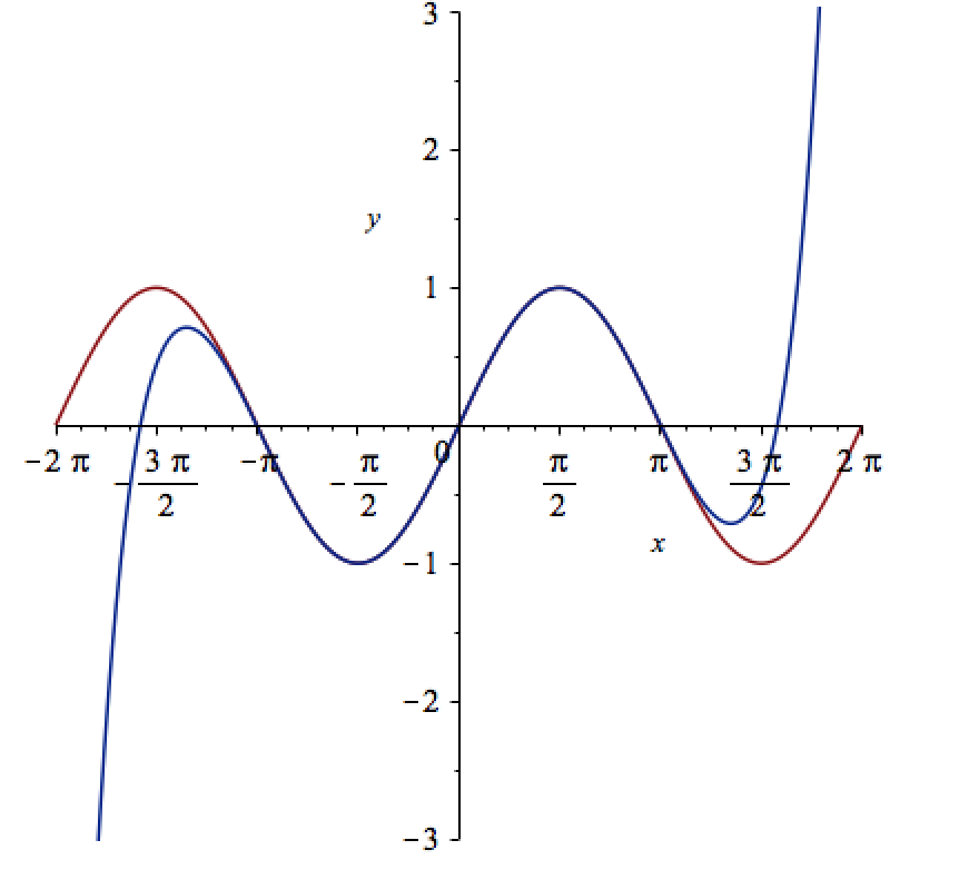
Let’s see how close this is to the sin(x) curve by plotting them both together

plot([sin(x), convert(series(sin(x), x = 0, 10), polynom)], x = -2*Pi .. 2*Pi, y = -3 .. 3);

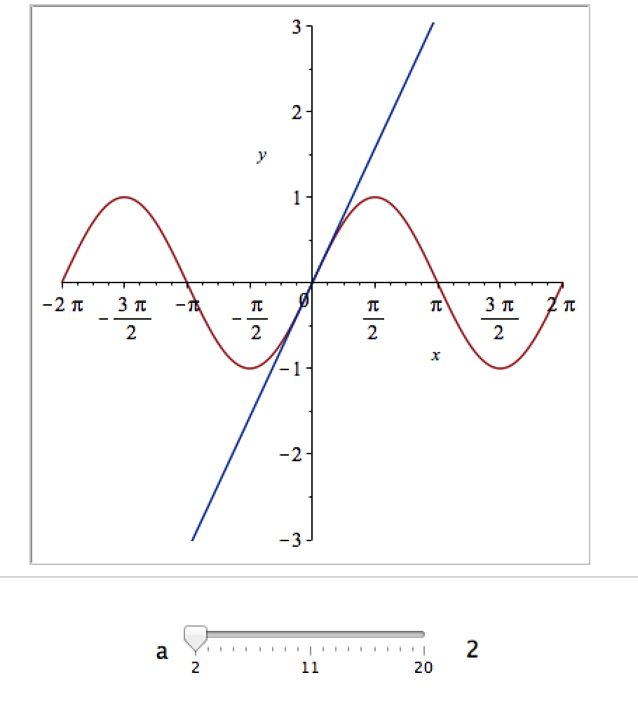
It would be nice if we could see how the approximation varies as we vary the number of terms in the expansion. Change the value 10 to a parameter a, pass the whole thing to the Explore function and we get an interactive widget.

Explore(plot([sin(x), convert(series(sin(x), x = 0, a), polynom)], x = -2*Pi .. 2*Pi, y = -3 .. 3), parameters = [a = 2 .. 20]);

Here’s a screenshot of it:

Adding extra parameters
It would also be nice to vary the point we expand around. Change the value 0 to b and add an extra parameter to Explore to get two sliders instead of one:

Explore(plot([sin(x), convert(series(sin(x), x = b, a), polynom)], x = -2*Pi .. 2*Pi, y = -3 .. 3), parameters = [a = 2 .. 20, b = -2*Pi .. 2*Pi]);

To see what this looks like, open the companion worksheet in Maple.

Adding labels to the sliders
We can change the labels on the sliders as follows

Explore(plot([sin(x), convert(series(sin(x), x = b, a), polynom)], x = -2*Pi .. 2*Pi, y = -3 .. 3), parameters = [[a = 2 .. 20, label = `Number Of Terms`], [b = -2*Pi .. 2*Pi, label = `Expansion location`]]);

To see what this looks like, open the companion worksheet in Maple.

Adding initial values
Finally, let’s set some starting values for each slider

Explore(plot([sin(x), convert(series(sin(x), x = b, a), polynom)], x = -2*Pi .. 2*Pi, y = -3 .. 3), parameters = [[a = 2 .. 20, label = `Number Of Terms`], [b = -2*Pi .. 2*Pi, label = `Expansion location`]], initialvalues = [a = 2, b = 1]);

The resulting interactive widget looks like this:

Not bad for one line of code!

Upload to the Maple Cloud

At The University of Sheffield, we are lucky because all of our staff and students have access to Maple on both university-owned and personally-owned equipment. If your audience isn’t as fortunate, they can access the resulting worksheet on the Maple Cloud.

I found these links a while ago and forgot to post them here. Some interesting insights.

• Wolfram Research compares Mathematica against Maple
• Maplesoft compares Maple against Mathematica

A question I get asked a lot is ‘How can I do nonlinear least squares curve fitting in X?’ where X might be MATLAB, Mathematica or a whole host of alternatives.  Since this is such a common query, I thought I’d write up how to do it for a very simple problem in several systems that I’m interested in

This is the Maple version. For other versions,see the list below

• Simple nonlinear least squares curve fitting in Julia
• Simple nonlinear least squares curve fitting in Mathematica
• Simple nonlinear least squares curve fitting in MATLAB
• Simple nonlinear least squares curve fitting in Python
• Simple nonlinear least squares curve fitting in R

The problem

xdata = -2,-1.64,-1.33,-0.7,0,0.45,1.2,1.64,2.32,2.9
ydata = 0.699369,0.700462,0.695354,1.03905,1.97389,2.41143,1.91091,0.919576,-0.730975,-1.42001

and you’d like to fit the function

using nonlinear least squares.  You’re starting guesses for the parameters are p1=1 and P2=0.2

For now, we are primarily interested in the following results:

• The fit parameters
• Sum of squared residuals

Future updates of these posts will show how to get other results such as confidence intervals. Let me know what you are most interested in.

Solution in Maple

Maple’s user interface is quite user friendly and it uses non-linear optimization routines from The Numerical Algorithms Group under the hood. Here’s the code to get the parameter values and sum of squares of residuals

with(Statistics):

xdata := Vector([-2, -1.64, -1.33, -.7, 0, .45, 1.2, 1.64, 2.32, 2.9], datatype = float):
ydata := Vector([.699369, .700462, .695354, 1.03905, 1.97389, 2.41143, 1.91091, .919576,  
  -.730975, -1.42001], datatype = float):
NonlinearFit(p1*cos(p2*x)+p2*sin(p1*x), xdata, ydata, x, initialvalues = [p1 = 1, p2 = .2], 
   output = [parametervalues, residualsumofsquares])

which gives the result

[[p1 = 1.88185090465902, p2 = 0.700229557992540], 0.05381269642]

Various other outputs can be specified in the output vector such as:

• solutionmodule
• degreesoffreedom
• leastsquaresfunction
• parametervalues
• parametervector
• residuals
• residualmeansquare
• residualstandarddeviation
• residualsumofsquares.

The meanings of the above are mostly obvious.  In those cases where they aren’t, you can look them up in the documentation link below.

Further documentation

The full documentation for Maple’s NonlinearFit command is at http://www.maplesoft.com/support/help/Maple/view.aspx?path=Statistics%2fNonlinearFit

Notes

I used Maple 17.02 on 64bit Windows to run the code in this post.

A colleague recently sent me this issue. Consider the following integral

Attempting to evaluate this with Mathematica 9 gives 0:

 f[a_, b_] := Exp[I*(a*x^3 + b*x^2)];
Integrate[f[a, b], {x, -Infinity, Infinity}, 
 Assumptions -> {a > 0, b \[Element] Reals}]

Out[2]= 0

So, for all valid values of a and b, Mathematica tells us that the resulting integral will be 0.

However, Let’s set a=1/3 and b=0 in the function f and ask Mathematica to evaluate that integral

In[3]:= Integrate[f[1/3, 0], {x, -Infinity, Infinity}]

Out[3]= (2*Pi)/(3^(2/3)*Gamma[2/3])

This is definitely not zero as we can see by numerically evaluating the result:

In[5]:=
(2*Pi)/(3^(2/3)*Gamma[2/3])//N

Out[5]= 2.23071

Similarly if we put a=1/3 and b=1 we get another non-zero result

In[7]:= Integrate[f[1/3, 1], {x, -Infinity, Infinity}] // InputForm

Out[7]=2*E^((2*I)/3)*Pi*AiryAi[-1]

In[8]:=
2*E^((2*I)/3)*Pi*AiryAi[-1]//N

Out[8]= 2.64453 + 2.08083 I

We are faced with a situation where Mathematica is disagreeing with itself.  On one hand, it says that the integral is 0 for all a and b but on the other it gives non-zero results for certain combinations of a and b.  Which result do we trust?

One way to proceed would be to use the NIntegrate[] function for the two cases where a and b are explicitly defined.  NIntegrate[] uses completely different algorithms from Integrate.  In particular it uses numerical rather than symbolic methods (apart from some symbolic pre-processing).

NIntegrate[f[1/3, 0], {x, -Infinity, Infinity}]

gives 2.23071 + 0. I and

NIntegrate[f[1/3, 1], {x, -Infinity, Infinity}]

gives 2.64453 + 2.08083 I

What we’ve shown here is that evaluating these integrals using numerical methods gives the same result as evaluating using symbolic methods and numericalizing the result.  This gives me some confidence that its the general, symbolic evaluation that’s incorrect and hence I can file a bug report with Wolfram Research.

Maple 17.01 on the general problem

Since my University has just got a site license for Maple, I wondered what Maple 17.01 would make of the general integral. Using Maple’s 1D input/output we get:

> myint := int(exp(I*(a*x^3+b*x^2)), x = -infinity .. infinity);

myint := (1/12)*3^(1/2)*2^(1/3)*((4/3)*Pi^(5/2)*(((4/27)*I)*b^3/a^2)^(1/3)*exp(((2/27)*I)*b^3/a^2)
*BesselI(-1/3, ((2/27)*I)*b^3/a^2)+((2/3)*I)*Pi^(3/2)*3^(1/2)*b*2^(2/3)
*hypergeom([1/2, 1], [2/3, 4/3],((4/27)*I)*b^3/a^2)/(-I*a)^(2/3)-(8/27)*2^(1/3)*Pi^(5/2)*b^2*
exp(((2/27)*I)*b^3/a^2)*BesselI(1/3, ((2/27)*I)*b^3/a^2)/((-I*a)^(4/3)*(((4/27)*I)*b^3/a^2)^(1/3)))
/(Pi^(3/2)*(-I*a)^(1/3))+(1/12)*3^(1/2)*2^(1/3)*((4/3)*Pi^(5/2)*(((4/27)*I)*b^3/a^2)
^(1/3)*exp(((2/27)*I)*b^3/a^2)*BesselI(-1/3, ((2/27)*I)*b^3/a^2)+((2/3)*I)*Pi^(3/2)*3^(1/2)*b*2^(2/3)
*hypergeom([1/2, 1], [2/3, 4/3], ((4/27)*I)*b^3/a^2)/(I*a)^(2/3)-(8/27)*2^(1/3)*Pi^(5/2)*b^2*
exp(((2/27)*I)*b^3/a^2)*BesselI(1/3, ((2/27)*I)*b^3/a^2)/((I*a)^(4/3)*(((4/27)*I)*b^3/a^2)^(1/3)))
/(Pi^(3/2)*(I*a)^(1/3))

That looks scary! To try to determine if it’s possibly a correct general result, let’s turn this expression into a function and evaluate it for values of a and b we already know the answer to.

>f := unapply(%, a, b):
>result1:=simplify(f(1/3,1));

result1 := (2/27)*3^(1/2)*Pi*exp((2/3)*I)*((-(1/3)*I)^(1/3)*3^(2/3)*(-1)^(1/6)*BesselI(-1/3, (2/3)*I)
+3*(-(1/3)*I)^(2/3)*BesselI(-1/3, (2/3)*I)+3*(-(1/3)*I)^(2/3)*BesselI(1/3, (2/3)*I)-BesselI(1/3, (2/3)*I)
*3^(1/3)*(-1)^(1/3))/(-(1/3)*I)^(2/3)

evalf(result1);
2.644532853+2.080831872*I

Recall that Mathematica returned 2*E^((2*I)/3)*Pi*AiryAi[-1]=2.64453 + 2.08083 I for this case. The numerical results agree to the default precision reported by both packages so I am reasonably confident that Maple’s general solution is correct.

Not so simple simplification?

I am also confident that Maple’s expression involving Bessel functions is equivalent to Mathematica’s expression involving the AiryAi function. I haven’t figured out, however, how to get Maple to automatically reduce the Bessel functions down to AiryAi. I can attempt to go the other way though. In Maple:

>convert(2*exp((2*I)/3)*Pi*AiryAi(-1),Bessel);

(2/3)*exp((2/3)*I)*Pi*(-1)^(1/6)*(-BesselI(1/3, (2/3)*I)*(-1)^(2/3)+BesselI(-1/3, (2/3)*I))

This is more compact than the Bessel function result I get from Maple’s simplify so I guess that Maple’s simplify function could have done a little better here.

Not so general general solution?

Maple’s solution of the general problem should be good for all a and b right?  Let’s try it with a=1/3, b=0

f(1/3,0);
Error, (in BesselI) numeric exception: division by zero

Uh-Oh! So it’s not valid for b=0 then! We know from Mathematica, however, that the solution for this particular case is (2*Pi)/(3^(2/3)*Gamma[2/3])=2.23071. Indeed, if we solve this integral directly in Maple, it agrees with Mathematica

>myint := int(exp(I*(1/3*x^3+0*x^2)), x = -infinity .. infinity);

myint := (2/9)*3^(5/6)*(-1)^(1/6)*Pi/GAMMA(2/3)-(2/9)*3^(5/6)*(-1)^(5/6)*Pi/GAMMA(2/3)

>simplify(myint);
(2/3)*3^(1/3)*Pi/GAMMA(2/3)

>evalf(myint);
2.230707052+0.*I

Going to back to the general result that Maple returned. Although we can’t calculate it directly, We can use limits to see what its value would be at a=1/3, b=0

>simplify(limit(f(1/3, x), x = 0));

(2/9)*Pi*3^(2/3)/((-(1/3)*I)^(1/3)*GAMMA(2/3)*((1/3)*I)^(1/3))

>evalf(%)

evalf(%);
2.230707053+0.1348486379e-9*I

The symbolic expression looks different and we’ve picked up an imaginary part that’s possibly numerical noise. Let’s use more numerical precision to see if we can make the imaginary part go away. 100 digits should do it

>evalf[100](%%);

2.230707051824495741427486519543450239771293806030489125938415383976032081571780278667202004477941904
-0.855678513686459467847075286617333072231119978694352241387724335424279116026690601018858453303153701e-100*I

Well, more precision has made the imaginary part smaller but it’s still there. No matter how much precision I use, it’s always there…getting smaller and smaller as I ramp up the level of precision.

What’s going on?

All I’m doing here is playing around with the same problem in two packages.  Does anyone have any further insights into some of the issues raised?

Maple has had support for NVidia GPUs since version 14 but I’ve not played with it much until recently.  Essentially I was put off by the fact that Maple’s CUDA package seemed to have support for only one function – Matrix-Matrix Multiplication. However, a recent conversation with a Maple developer changed my mind.

It is true that only MatrixMatrixMultiply has been accelerated but when you flip the CUDA switch in Maple, every function in the LinearAlgebra package that calls MatrixMatrixMultiply also gets accelerated.  This leads to the possibility of a lot of speed-ups for very little work.

So, this morning I thought I would take a closer look using my laptop.  Let’s start by timing how long it takes the CPU to multiply two 4000 by 4000 double precision matrices

with(LinearAlgebra):
CUDA:-Enable(false):
CUDA:-IsEnabled();
a := RandomMatrix(4000, datatype = float[8]):
b := RandomMatrix(4000, datatype = float[8]):
t := time[real]():
c := a.b:
time[real]()-t

The exact time varied a little from run to run but 3.76 seconds is a typical result. I’m only feeling my way at this stage so not doing any proper benchmarking.

To do this calculation on the GPU, all I need to do is change the line

CUDA:-Enable(false):

to

CUDA:-Enable(true):

like so

with(LinearAlgebra):
CUDA:-Enable(true):
CUDA:-IsEnabled();
a := RandomMatrix(4000, datatype = float[8]):
b := RandomMatrix(4000, datatype = float[8]):
t := time[real]():
c := a.b:
time[real]()-t

Typical execution time was 8.37 seconds so the GPU version is more than 2 times slower than the CPU version on my machine.

Trying different matrix sizes

Not wanting to admit defeat after just a single trial, I timed the above code using different matrix sizes.  Here are the results

• 1000 by 1000: CPU=0.07 seconds GPU=0.17 seconds
• 2000 by 2000: CPU=0.53 seconds GPU=1.07 seconds
• 4000 by 4000: CPU=3.76 seconds GPU=8.37 seconds
• 5000 by 5000: CPU=7.44 seconds GPU=19.48 seconds

Switching to single precision

GPUs do much better with single precision numbers so I had a try with those too.  All you need to do is change

datatype = float[8]

to

datatype = float[4]

in the above code. The results are:

• 1000 by 1000: CPU=0.03 seconds GPU=0.07 seconds
• 2000 by 2000: CPU=0.35 seconds GPU=0.66 seconds
• 4000 by 4000: CPU=1.86 seconds GPU=2.37 seconds
• 5000 by 5000: CPU=3.81 seconds GPU=5.2 seconds

So the GPU loses in single precision mode too on my hardware.  If I can’t get a speedup with MatrixMatrixMultiply on my system then there is no point in exploring all of the other LinearAlgebra routines since all of them will be slower when moving to CUDA acceleration.

I guess that in this case, my CPU is too powerful and my GPU is too wimpy to see the acceleration I was hoping for.

Thanks to Maplesoft for providing me with a review copy of Maple 15.

Test System Specification

• Laptop model: Dell XPS L702X
• CPU: Intel Core i7-2630QM @2Ghz software overclockable to 2.9Ghz. 4 physical cores but total 8 virtual cores due to Hyperthreading.
• GPU: GeForce GT 555M with 144 CUDA Cores.  Graphics clock: 590Mhz.  Processor Clock:1180 Mhz. 3072 Mb DDR3 Memeory
• RAM: 8 Gb
• OS: Windows 7 Home Premium 64 bit.
• Maple 15

My attention was recently drawn to a Google+ post by JerWei Zhang where he evaluates 2^3^4 in various packages and notes that they don’t always agree.  For example, in MATLAB 2010a we have 2^3^4 = 4096 which is equivalent to putting (2^3)^4 whereas Mathematica 8 gives 2^3^4 = 2417851639229258349412352 which is the same as putting 2^(3^4).  JerWei’s post gives many more examples including Excel, Python and Google and the result is always one of these two (although to varying degrees of precision).

What surprised me was the fact that they disagreed at all since I thought that the operator precendence rules were an agreed standard across all software packages.  In this case I’d always use brackets since _I_ am not sure what the correct interpretation of 2^3^4 should be but I would have taken it for granted that there is a standard somewhere and that all of the big hitters in the numerical world would adhere to it.

Looks like I was wrong!

Typical…I leave my iPad at home and this happens

I can’t WAIT to try this out.  Blog post from Maplesoft about it at http://www.mapleprimes.com/maplesoftblog/127071-Maple-And-The-IPad?sp=127071

May I be the first to ask “When is an Android version coming out?”

Updated January 4th 2011

It is becoming increasingly common for programmers to make use of GPUs (Graphical Processing Units) to speed up their programs substantially.  There are three major low-level programming libraries that allow you to do this in languages such as C; namely CUDA, OpenCL and Microsoft DirectCompute.  Of these three, CUDA is the most developed but it only works on Nvidia graphics cards.

I am often asked if the major commercial math packages support GPU computing and I find myself writing the same summary email over and over again.  So, here is a very brief breakdown of what is currently on offer.  I plan to expand the information contained in this page over time so if you have any information about GPU computing in these packages then let me know.

MATLAB

Core MATLAB contains no support for GPU computing but several organizations (including The Mathworks themselves) have produced add-on toolboxes that add such support:

• Jacket – This is a product from a company called AccelerEyes and is possibly the most advanced and well developed GPU solution for MATLAB currently available.  As of version 2.0 it supports both OpenCL and CUDA frameworks.
• The Mathworks’ Parallel Computing Toolbox (PCT) – If you want to do your MATLAB GPU computing the officially supported way then this is the product you need.  As a bonus, it also allows you to make better use of the multicore processor that almost certainly resides in your machine.  Like many of the offerings on this page, only the CUDA framework is supported so you are out of luck if you don’t have an NVidia graphics card.  Even if you do have an NVidia graphics card then you still might be out of luck since the PCT only supports cards that have compute level 1.3 or above (i.e. double precision only).
• CULA is a set of GPU-accelerated linear algebra libraries utilizing the NVIDIA CUDA parallel computing architecture and it has a MATLAB interface.
• GPUmat – This product is completely free but is less developed than the commercial offerings above.  Again. it is CUDA only
• OpenCL toolbox – The only OpenCL solution for MATLAB I could find.  It is free but development seems to have stalled.

Mathematica

Mathematica 8 has support for both CUDA and OpenCL built in so no need for any add-ons.  Furthermore, it supports both single and double precision GPUs so you can experiment with GPU computing on older, cheaper cards.

Maple

Maple has had some CUDA-only GPU support since version 14.  On the face of it, the CUDA package only appears to contain one accelerated function–Matrix-Matrix multiplication– but when you load this function it accelerates many functions that use matrix-matrix multiply internally.  I’ve never found a definitive list of such functions though.

Mathcad

Mathcad 15 and Mathcad Prime have no support for GPU enhanced computing.