
Archive for the ‘Open Source’ Category
Feel free to discuss and contribute to this article over at the corresponding GitHub repo.
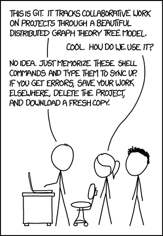
Many people suggest that you should use version control as part of your scientifc workflow. This is usually quickly followed up by recommendations to learn git and to put your project on GitHub. Learning and doing all of this for the first time takes a lot of effort. Alongside all of the recommendations to learn these technologies are horror stories telling how difficult it can be and memes saying that no one really knows what they are doing!
There are a lot of reasons to not embrace the git but there are even more to go ahead and do it. This is an attempt to convince you that it’s all going to be worth it alongside a bunch of resources that make it easy to get started and academic papers discussing the issues that version control can help resolve.
This document will not address how to do version control but will instead try to answer the questions what you can do with it and why you should bother. It was inspired by a conversation on twitter.
Improvements to individual workflow
Ways that git and GitHub can help your personal computational workflow – even if your project is just one or two files and you are the only person working on it.
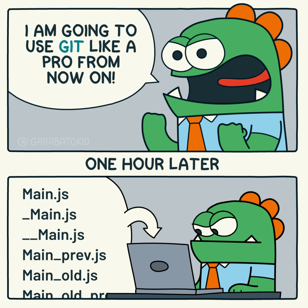
Fixing filename hell
Is this a familiar sight in your working directory?
mycode.py
mycode_jane.py
mycode_ver1b.py
mycode_ver1c.py
mycode_ver1b_january.py
mycode_ver1b_january_BROKEN.py
mycode_ver1b_january_FIXED.py
mycode_ver1b_january_FIXED_for_supervisor.py
For many people, this is just the beginning. For a project that has existed long enough there might be dozens or even hundreds of these simple scripts that somehow define all of part of your computational workflow. Version control isn’t being used because ‘The code is just a simple script developed by one person’ and yet this situation is already becoming the breeding ground for future problems.
- Which one of these files is the most up to date?
- Which one produced the results in your latest paper or report?
- Which one contains the new work that will lead to your next paper?
- Which ones contain deep flaws that should never be used as part of the research?
- Which ones contain possibly useful ideas that have since been removed from the most recent version?
Applying version control to this situation would lead you to a folder containing just one file
mycode.pyAll of the other versions will still be available via the commit history. Nothing is ever lost and you’ll be able to effectively go back in time to any version of mycode.py you like.
A single point of truth
I’ve even seen folders like the one above passed down generations of PhD students like some sort of family heirloom. I’ve seen labs where multple such folders exist across a dozen machines, each one with a mixture of duplicated and unique files. That is, not only is there a confusing mess of files in a folder but there is a confusing mess of these folders!
This can even be true when only one person is working on a project. Perhaps you have one version of your folder on your University HPC cluster, one on your home laptop and one on your work machine. Perhaps you email zipped versions to yourself from time to time. There are many everyday events that can lead to this state of affairs.
By using a GitHub repository you have a single point of truth for your project. The latest version is there. All old versions are there. All discussion about it is there.
Everything…one place.
The power of this simple idea cannot be overstated. Whenever you (or anyone else) wants to use or continue working on your project, it is always obvious where to go. Never again will you waste several days work only to realise that you weren’t working on the latest version.
Keeping track of everything that changed
The latest version of your analysis or simulation is different from the previous one. Thanks to this, it may now give different results today compared to yesterday. Version control allows you to keep track of everything that changed between two versions. Every line of code you added, deleted or changed is highlighted. Combined with your commit messages where you explain why you made each set of changes, this forms a useful record of the evolution of your project.
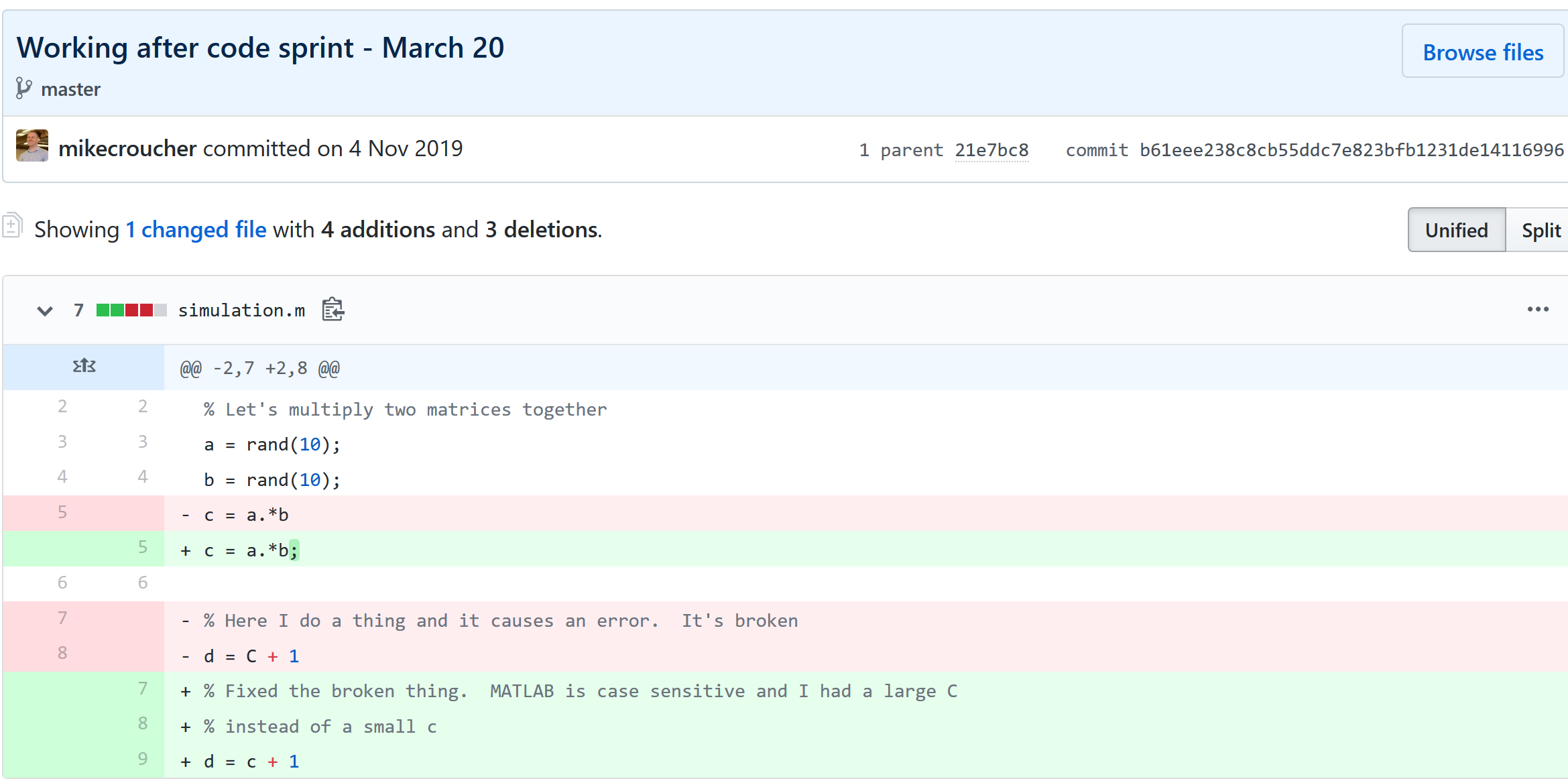
It is possible to compare the differences between any two commits, not just two consecutive ones which allows you to track the evolution of your project over time.
Always having a working version of your project
Ever noticed how your collaborator turns up unnanounced just as you are in the middle of hacking on your code. They want you to show them your simulation running but right now its broken! You frantically try some of the other files in your folder but none of them seem to be the version that was working last week when you sent the report that moved your collaborator to come to see you.
If you were using version control you could easily stash your current work, revert to the last good commit and show off your work.
Tracking down what went wrong
You are always changing that script and you test it as much as you can but the fact is that the version from last year is giving correct results in some edge case while your current version is not. There are 100 versions between the two and there’s a lot of code in each version! When did this edge case start to go wrong?
With git you can use git bisect to help you track down which commit started causing the problem which is the first step towards fixing it.

Providing a back up of your project
Try this thought experiment: Your laptop/PC has gone! Fire, theft, dead hard disk or crazed panda attack.

It, and all of it’s contents have vanished forever. How do you feel? What’s running through your mind? If you feel the icy cold fingers of dread crawling up your spine as you realise Everything related to my PhD/project/life’s work is lost then you have made bad life choices. In particular, you made a terrible choice when you neglected to take back ups.
Of course there are many ways to back up a project but if you are using the standard version control workflow, your code is automatically backed up as a matter of course. You don’t have to remember to back things up, back-ups happen as a natural result of your everyday way of doing things.
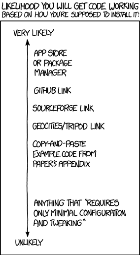
Making your project easier to find and install
There are dozens of ways to distribute your software to someone else. You could (HORRORS!) email the latest version to a colleuage or you could have a .zip file on your web site and so on.
Each of these methods has a small cognitive load for both recipient and sender. You need to make sure that you remember to update that .zip file on your website and your user needs to find it. I don’t want to talk about the email case, it makes me too sad. If you and your collaborator are emailing code to each other, please stop. Think of the children!
One great thing about using GitHub is that it is a standardised way of obtaining software. When someone asks for your code, you send them the URL of the repo. Assuming that the world is a better place and everyone knows how to use git, you don’t need to do anything else since the repo URL is all they need to get your code. a git clone later and they are in business.
Additionally, you don’t need to worry abut remembering to turn your working directory into a .zip file and uploading it to your website. The code is naturally available for download as part of the standard workflow. No extra thought needed!
In addition to this, some popular computational environments now allow you to install packages directly from GitHub. If, for example, you are following standard good practice for building an R package then a user can install it directly from your GitHub repo from within R using the devtools::install_github() function.
Automatically run all of your tests
You’ve sipped of the KoolAid and you’ve been writing unit tests like a pro. GitHub allows you to link your repo with something called Continuous Integration (CI) that helps maximise the utility of those tests.
Once its all set up the CI service runs every time you, or anyone else, makes a commit to your project. Every time the CI service runs, a virtual machine is created from scratch, your project is installed into it and all of your tests are run with any failures reported.
This gives you increased confidence that everything is OK with your latest version and you can choose to only accept commits that do not break your testing framework.
Collaboration and Community
How git and GitHub can make it easier to collaborate with others on computational projects.
Control exactly who can see your work
‘I don’t want to use GitHub because I want to keep my project private’ is a common reason given to me for not using the service. The ability to create private repositories has been free for some time now (Price plans are available here https://github.com/pricing) and you can have up to 3 collaborators on any of your private repos before you need to start paying. This is probably enough for most small academic projects.
This means that you can control exactly who sees your code. In the early stages it can be just you. At some point you let a couple of trusted collaborators in and when the time is right you can make the repo public so everyone can enjoy and use your work alongside the paper(s) it supports.
Faciliate discussion about your work
Every GitHub repo comes with an Issues section which is effectively a discussion forum for the project. You can use it to keep track of your project To-Do list, bugs, documentation discussions and so on. The issues log can also be integrated with your commit history. This allows you to do things like git commit -m "Improve the foo algorithm according to the discussion in #34" where #34 refers to the Issue discussion where your collaborator pointed out
Allow others to contribute to your work
You have absolute control over external contributions! No one can make any modifications to your project without your explicit say-so.
I start with the above statement because I’ve found that when explaining how easy it is to collaborate on GitHub, the first question is almost always ‘How do I keep control of all of this?’
What happens is that anyone can ‘fork’ your project into their account. That is, they have an independent copy of your work that is clearly linked back to your original. They can happily work away on their copy as much as they like – with no involvement from you. If and when they want to suggest that some of their modifications should go into your original version, they make a ‘Pull Request’.
I emphasised the word ‘Request’ because that’s exactly what it is. You can completely ignore it if you want and your project will remain unchanged. Alternatively you might choose to discuss it with the contributor and make modifications of your own before accepting it. At the other end of the spectrum you might simply say ‘looks cool’ and accept it immediately.
Congratulations, you’ve just found a contributing collaborator.
Reproducible research
How git and GitHub can contribute to improved reproducible research.
Simply making your software available
A paper published without the supporting software and data is (much!) harder to reproduce than one that has both.
Making your software citable
Most modern research cannot be done without some software element. Even if all you did was run a simple statistical test on 20 small samples, your paper has a data and software dependency. Organisations such as the Software Sustainability Institute and the UK Research Software Engineering Association (among many others) have been arguing for many years that such software and data dependencies should be part of the scholarly record alongside the papers that discuss them. That is, they should be archived and referenced with a permanent Digital Object Identifier (DOI).
Once your code is in GitHub, it is straightforward to archive the version that goes with your latest paper and get it its own DOI using services such as Zenodo. Your University may also have its own archival system. For example, The University of Sheffield in the UK has built a system called ORDA which is based on an institutional Figshare instance which allows Sheffield academics to deposit code and data for long term archival.
Which version gave these results?
Anyone who has worked with software long enough knows that simply stating the name of the software you used is often insufficient to ensure that someone else could reproduce your results. To help improve the odds, you should state exactly which version of the software you used and one way to do this is to refer to the git commit hash. Alternatively, you could go one step better and make a GitHub release of the version of your project used for your latest paper, get it a DOI and cite it.
This doesn’t guarentee reproducibility but its a step in the right direction. For extra points, you may consider making the computational environment reproducible too (e.g. all of the dependencies used by your script – Python modules, R packages and so on) using technologies such as Docker, Conda and MRAN but further discussion of these is out of scope for this article.
Building a computational environment based on your repository
Once your project is on GitHub, it is possible to integrate it with many other online services. One such service is mybinder which allows the generation of an executable environment based on the contents of your repository. This makes your code immediately reproducible by anyone, anywhere.
Similar projects are popping up elsewhere such as The Littlest JupyterHub deploy to Azure button which allows you to add a button to your GitHub repo that, when pressed by a user, builds a server in their Azure cloud account complete with your code and a computational environment specified by you along with a JupterHub instance that allows them to run Jupyter notebooks. This allows you to write interactive papers based on your software and data that can be used by anyone.
Complying with funding and journal guidelines
When I started teaching and advocating the use of technologies such as git I used to make a prediction These practices are so obviously good for computational research that they will one day be mandated by journal editors and funding providers. As such, you may as well get ahead of the curve and start using them now before the day comes when your funding is cut off because you don’t. The resulting debate was usually good fun.
My prediction is yet to come true across the board but it is increasingly becoming the case where eyebrows are raised when papers that rely on software are published don’t come with the supporting software and data. Research Software Engineers (RSEs) are increasingly being added to funding review panels and they may be Reviewer 2 for your latest paper submission.
Other uses of git and GitHub for busy academics
It’s not just about code…..
- Build your own websites using GitHub pasges. Every repo can have its own website served directly from GitHub
- Put your presentations on GitHub. I use reveal.js combined with GitHub pages to build and serve my presentations. That way, whenever I turn up at an event to speak I can use whatever computer is plugged into the projector. No more ‘I don’t have the right adaptor’ hell for me.
- Write your next grant proposal. Use Markdown, LaTex or some other git-friendly text format and use git and GitHub to collaboratively write your next grant proposal
The movie below is a visualisation showing how a large H2020 grant proposal called OpenDreamKit was built on GitHub. Can you guess when the deadline was based on the activity?
Further Resources
Further discussions from scientific computing practitioners that discuss using version control as part of a healthy approach to scientific computing
- Good Enough Practices in Scientific Computing –
- Is Your Research Software Correct? – A presentation from Mike Croucher discussing what can go wrong in computational research and what practices can be adopted to do help us do better
- The Turing Way A handbook of good practice in data science brought to you from the Alan Turning Institute
- A guide to reproducible code in ecology and evolution – A handbook from the British Ecological Society that discusses version control as part of general good practice
Learning version control
Convinced? Want to start learning? Let’s begin!
- Git lesson from Software Carpentry – A free, community written tutorial on the basics of git version control
Graphical User Interfaces to git
If you prefer not to use the command line, try these
My stepchildren are pretty good at mathematics for their age and have recently learned about Pythagora’s theorem
$c=\sqrt{a^2+b^2}$
The fact that they have learned about this so early in their mathematical lives is testament to its importance. Pythagoras is everywhere in computational science and it may well be the case that you’ll need to compute the hypotenuse to a triangle some day.
Fortunately for you, this important computation is implemented in every computational environment I can think of!
It’s almost always called hypot so it will be easy to find.
Here it is in action using Python’s numpy module
import numpy as np
a = 3
b = 4
np.hypot(3,4)

5
When I’m out and about giving talks and tutorials about Research Software Engineering, High Performance Computing and so on, I often get the chance to mention the hypot function and it turns out that fewer people know about this routine than you might expect.
Trivial Calculation? Do it Yourself!
Such a trivial calculation, so easy to code up yourself! Here’s a one-line implementation
def mike_hypot(a,b):
    return(np.sqrt(a*a+b*b))
In use it looks fine
mike_hypot(3,4)

5.0
Overflow and Underflow
I could probably work for quite some time before I found that my implementation was flawed in several places. Here’s one
mike_hypot(1e154,1e154)

inf
You would, of course, expect the result to be large but not infinity. Numpy doesn’t have this problem
np.hypot(1e154,1e154)

1.414213562373095e+154
My function also doesn’t do well when things are small.
a = mike_hypot(1e-200,1e-200)

0.0
but again, the more carefully implemented hypot function in numpy does fine.
np.hypot(1e-200,1e-200)

1.414213562373095e-200
Standards Compliance
Next up — standards compliance. It turns out that there is a an official standard for how hypot implementations should behave in certain edge cases. The IEEE-754 standard for floating point arithmetic has something to say about how any implementation of hypot handles NaNs (Not a Number) and inf (Infinity).
It states that any implementation of hypot should behave as follows (Here’s a human readable summary https://www.agner.org/optimize/nan_propagation.pdf)
hypot(nan,inf) = hypot(inf,nan) = inf
numpy behaves well!
np.hypot(np.nan,np.inf)

inf

np.hypot(np.inf,np.nan)

inf
My implementation does not
mike_hypot(np.inf,np.nan)

nan
So in summary, my implementation is
- Wrong for very large numbers
- Wrong for very small numbers
- Not standards compliant
That’s a lot of mistakes for one line of code! Of course, we can do better with a small number of extra lines of code as John D Cook demonstrates in the blog post What’s so hard about finding a hypotenuse?
Hypot implementations in production
Production versions of the hypot function, however, are much more complex than you might imagine. The source code for the implementation used in openlibm (used by Julia for example) was 132 lines long last time I checked. Here’s a screenshot of part of the implementation I saw for prosterity. At the time of writing the code is at https://github.com/JuliaMath/openlibm/blob/master/src/e_hypot.c
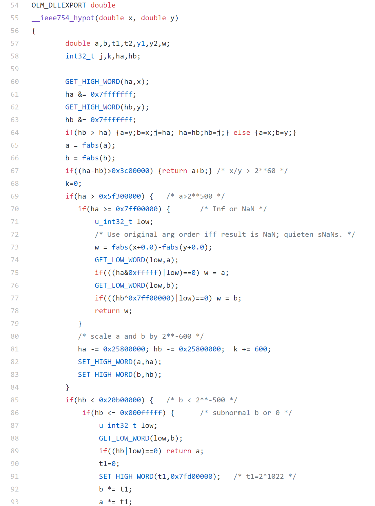
That’s what bullet-proof, bug checked, has been compiled on every platform you can imagine and survived code looks like.
There’s more!
Active Research
When I learned how complex production versions of hypot could be, I shouted out about it on twitter and learned that the story of hypot was far from over!
The implementation of the hypot function is still a matter of active research! See the paper here https://arxiv.org/abs/1904.09481

Is Your Research Software Correct?
Given that such a ‘simple’ computation is so complicated to implement well, consider your own code and ask Is Your Research Software Correct?.
A colleague recently sent me the following code snippet in R
> a=c(1,2,3,40)
> b=a[1:10]
> b
[1]  1  2  3 40 NA NA NA NA NA NA
The fact that R didn’t issue a warning upset him since exceeding array bounds, as we did when we created b, is usually a programming error.
I’m less concerned and simply file the above away in an area of my memory entitled ‘Odd things to remember about R’ — I find that most programming languages have things that look odd when you encounter them for the first time. With that said, I am curious as to why the designers of R thought that the above behaviour was a good idea.
Does anyone have any insights here?
Octave is a free, open source language for numerical computing that is mostly compatible with MATLAB. For years, the official Octave project has been strictly command-line only which puts many users off — particularly those who were used to the graphical user interface (GUI) of MATLAB. Unofficial GUIs have come and gone over the years but none of them were fully satisfactory for one reason or another.
As of the 3.8 release of Octave on 31st December 2013, this all changed when Octave started shipping with its own, official GUI. It is currently considered as ‘experimental’ by the Octave team and is obviously rough around the edges here and there but it is already quite usable.
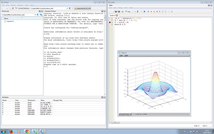
The system includes
- An editor with syntax highlighting and code folding
- A debugger
- A file browser and workspace viewer
- The ability to hide and move different elements of the GUI around (e.g. you could swap the positions of the workspace and File Browser, or tear-off the editor into its own Window)
- A documentation browser
- The Octave command window
I’ve spent an hour or so playing with it today and like it a lot!
Thanks to Júlio Hoffimann Mendes who let me know about this new release.
I work for The University of Manchester where, among other things, I assist in the support of various high performance and high throughput computing systems. Exchanges such as the following are, sadly, becoming all too commonplace
Researcher: “Hi, I have an embarrassingly parallel research problem that needs a lot of compute resource. Can you help?”
Support: “Almost certainly, you could have access to our 2500 core Condor pool or maybe our 2000 core HPC system or any number of smaller systems depending on the department you are in. Let’s meet to discuss your requirements in more detail”
Researcher: “Sounds great. I am using [insert expensive commercial package here], could we install that on your systems?”
Support: “Not unless you pay a HUGE amount of money because you’ll need dozens or maybe hundreds of licenses. The licenses will cost more than our machines! Could you use [insert open source equivalent here] instead?”
Researcher: “A member of your team suggested that about 2 years ago but [insert expensive commercial package here] is easier to use, looks pretty and a single license didn’t seem all that expensive. It’ll take me ages to convert to [insert open source equivalent here]. Instead of splitting the job up and spreading it around lots of machines, can’t I just run it on a faster machine?”
Support: “Sorry but parallelism is the only real game in town when it comes to making stuff faster these days. I’m afraid that you’ll have to convert to [insert open source equivalent here], open your chequebook or wait until 2076 for your results to complete on your workstation.”
The moral of the story is that if you want your compute to scale, you need to ensure that your licensing scales too.
Apple make a big deal out of the fact that their app stores for iPhone and iPad contain thousands upon thousands of apps (or applications for relative oldies such as myself). Some of them are free of change, many of them cost money but I got to wondering how many of them were open source.
When I say ‘open source’ here I mean ‘The source code is available’. If there is a recognised license attached to the source code (such as GPL or BSD) then all the better. So, what do we have?
Possibly the the best list of iOS open source software I have found is available at maniacdev.com which, at the time of writing, includes 42 different applications complete with iTunes links and the all important links to source code. Another useful resource is open.iphonedev.com which is a regularly updated directory of open source apps and libraries for iOS. There’s some great stuff available including Battle for Wesnorth, SCI-15C Scientific calculator and TuxRider (based on Tux Racer).
Free as in Speech but not always Free as in Beer
One of the things you’ll notice about iOS open source apps is that they often cost money and sometimes quite a lot which is in stark contrast to what you may be used to. For example, Battle for Wesnorth can be had for no money at all on platforms such as Linux and Windows but the iPad version costs $5.99 at the time of writing. The more serious, SCI-15C Scientific calculator costs $19.99 right now which is rather steep for any iPhone app let alone an open source one.
Charging money for open source software may upset some people but doing so is usually not against the terms and conditions of the underlying license. The Free Software Foundation (inventors of the GPL, one of the most popular forms of open source license) has the following to say on the matter (original source)
“Free software” is a matter of liberty, not price. To understand the concept, you should think of “free” as in “free speech,” not as in “free beer.
Personally, I am happy to pay a few dollars for the iPad version of an open-source app if the developer has done a good job of the port. What does surprise me, however, is that it seems like no one has taken the source-code of these apps, recompiled them and then released free-of-charge versions on the app store. This wouldn’t be against the license conditions of licenses such as the GPL so why hasn’t it been done? I wouldn’t do it because I feel that it would be unfair to the developer of the iOS version but I would be surprised if everyone felt this way.
What’s next?
There are many open source applications that I’d love to see ported to iPad. Here’s my top three wants:
- FreeCiv (An Android port is on the way!)
- Gnuplot (This was done for Windows Mobile ages ago – see my review of it here)
- Octave (The iPad is more powerful than the laptop I did my PhD on. Plenty for basic Octave use)
Over to you….What do you think of the state of open source software on iPhone and iPad? Which applications would you most like to see ported? What are your favourite open source apps?
Update: 9th March 2011. Apparently, many of the open source applications currently available on the App store today violate the terms of licenses such as the GPL. The Inquirer has more details.
Christmas isn’t all that far away so I thought that it was high time that I wrote my Christmas list for mathematical software developers and vendors. All I want for christmas is….
Mathematica
- A built in ternary plot function would be nice
- Ship workbench with the main product please
- An iPad version of Mathematica Player
MATLAB
- Merge the parallel computing toolbox with core MATLAB. Everyone uses multicore these days but only a few can feel the full benefit in MATLAB. The rest are essentially second class MATLAB citizens muddling by with a single core (most of the time)
- Make the mex interface thread safe so I can more easily write parallel mex files
Maple
- More CUDA accelerated functions please. I was initially excited by your CUDA package but then discovered that it only accelerated one function (Matrix Multiply). CUDA accelerated Random Number Generators would be nice along with fast Fourier transforms and a bit more linear algebra.
MathCAD
- Release Mathcad Prime.
- Mac and Linux versions of Mathcad. Maple,Mathematica and MATLAB have versions for all 3 platforms so why don’t you?
NAG Library
- Produce vector versions of functions like g01bk (poisson distribution function). They might not be needed in Fortran or C code but your MATLAB toolbox desperately needs them
- A Mac version of the MATLAB toolbox. I’ve got users practically begging for it :)
- A NAG version of the MATLAB gamfit command
Octave
- A just in time compiler. Yeah, I know, I don’t ask for much huh ;)
- A faster pdist function (statistics toolbox from Octave Forge). I discovered that the current one is rather slow recently
SAGE Math
- A Locator control for the interact function. I still have a bounty outstanding for the person who implements this.
- A fully featured, native windows version. I know about the VM solution and it isn’t suitable for what I want to do (which is to deploy it on around 5000 University windows machines to introduce students to one of the best open source maths packages)
SMath Studio
- An Android version please. Don’t make it free – you deserve some money for this awesome Mathcad alternative.
SpaceTime Mathematics
- The fact that you give the Windows version away for free is awesome but registration is a pain when you are dealing with mass deployment. I’d love to deploy this to my University’s Windows desktop image but the per-machine registration requirement makes it difficult. Most large developers who require registration usually come up with an alternative mechanism for enterprise-wide deployment. You ask schools with more than 5 machines to link back to you. I want tot put it on a few thousand machines and I would happily link back to you from several locations if you’ll help me with some sort of volume license. I’ll also give internal (and external if anyone is interested) seminars at Manchester on why I think Spacetime is useful for teaching mathematics. Finally, I’d encourage other UK University applications specialists to evaluate the software too.
- An Android version please.
How about you? What would you ask for Christmas from your favourite mathematical software developers?
MATLAB contains a function called pdist that calculates the ‘Pairwise distance between pairs of objects’. Typical usage is
X=rand(10,2);
dists=pdist(X,'euclidean');
It’s a nice function but the problem with it is that it is part of the Statistics Toolbox and that costs extra. I was recently approached by a user who needed access to the pdist function but all of the statistics toolbox license tokens on our network were in use and this led to the error message
??? License checkout failed.
License Manager Error -4
Maximum number of users for Statistics_Toolbox reached.
Try again later.
To see a list of current users use the lmstat utility or contact your License Administrator
One option, of course, is to buy more licenses for the statistics toolbox but there is another way. You may have heard of GNU Octave, a free,open-source MATLAB-like program that has been in development for many years. Well, Octave has a sister project called Octave-Forge which aims to provide a set of free toolboxes for Octave. It turns out that not only does Octave-forge contain a statistics toolbox but that toolbox contains an pdist function. I wondered how hard it would be to take Octave-forge’s pdist function and modify it so that it ran on MATLAB.
Not very! There is a script called oct2mat that is designed to automate some of the translation but I chose not to use it – I prefer to get my hands dirty you see. I named the resulting function octave_pdist to help clearly identify the fact that you are using an Octave function rather than a MATLAB function. This may matter if one or the other turns out to have bugs. It appears to work rather nicely:
dists_oct = octave_pdist(X,'euclidean');
% let's see if it agrees with the stats toolbox version
all( abs(dists_oct-dists)<1e-10)

ans =
     1
Let’s look at timings on a slightly bigger problem.
>> X=rand(1000,2);
>> tic;matdists=pdist(X,'euclidean');toc
Elapsed time is 0.018972 seconds.
>> tic;octdists=octave_pdist(X,'euclidean');toc
Elapsed time is 6.644317 seconds.
Uh-oh! The Octave version is 350 times slower (for this problem) than the MATLAB version. Ouch! As far as I can tell, this isn’t down to my dodgy porting efforts, the original Octave pdist really does take that long on my machine (Ubuntu 9.10, Octave 3.0.5).
This was far too slow to be of practical use and we didn’t want to be modifying algorithms so we ditched this function and went with the NAG Toolbox for MATLAB instead (routine g03ea in case you are interested) since Manchester effectively has an infinite number of licenses for that product.
If,however, you’d like to play with my MATLAB port of Octave’s pdist then download it below.
- octave_pdist.m makes use of some functions in the excellent NaN Toolbox so you will need to download and install that package first.
Did you make any New Year’s resolutions this year? If you did then who will they help? Just you? Your family? Your students? The whole world? If I am being honest then I have to say that most of the new-year’s resolutions I have made over the years tend to focus on myself because at my very core I am a bit selfish. So, my resolutions tend to be things like “I want to get fitter”, “I’ll not stay late at work so much” or “I want to learn more Python programming.”
If I keep these resolutions then I’m going to be fitter, more knowledgeable and have a better work-life balance. So far so selfish!
Over the last few days though I have made a rather different sort of new-years resolution. Yes, I admit that it’s a bit late but why limit change to an essentially arbitrary date? My new new year’s resolution is to give a little back to the community that has given me so much – the community of organisations and individuals who provide me with software – either for free or for such a trivial amount of money that it may as well be free.
Now I am not a rich man so I can’t give away great wads of cash and although I am a programmer I have neither the time nor the knowledge to provide significant amounts of code to any particualr project. So what can I do?
Donations
Well, although I am not minted, I can easily afford the occasional small donation or two so I will start making them. It’s already begun with my Sage bounty hunt and will continue with other projects over the year. Another small donation I made recently was to buy the ‘Premium’ version of Aldiko – a great ebook reader for Android smartphones. Aldiko is a free piece of software, has been downloaded by tens of thousands of users and is used by me on an almost daily basis. I noticed that they had a ‘Premium’ version available for $1.99 but it turns out that it is identical to the free version. The $1.99 simply represents a donation to the developers and it’s a donation I made without hesitation. Doing the right thing for less than two dollars – getting the warm fuzzies has never been easier!
Bug reports and feedback
Thanks to my job and to running Walking Randomly I get to see how researchers, teachers, students and average joes use mathematical software quite a lot. I get told about bugs, about feature wish lists, about gripes with licensing, performance issues…the list goes on and on. The best way to get bugs fixed is to report them – first tell the developers and, if the bug is interesting/severe enough, tell the world. I do this plenty with commercial software but I am going to make the effort more with free software from now on. Feedback is part of the lifeblood of free software and developers need both the good and the bad.
Did you try out Octave, Maxima, Sage or Smath Studio and it didn’t work out? Why didn’t it? What did these packages have missing that forced you to turn to alternatives? Try to be specific; saying ‘I tried it and it sucks’ is a rubbish piece of feedback because it’s just an opinion and gives the developers nothing to do. Saying something like ‘I tried to calculate XYZ and it gave the following incorrect result whereas it should have given ABC’ is MUCH more productive.
Tutorials, examples and documentation
One comment I have heard over and over again from people who have tried free mathematical software and then turned their back on it is that the ‘documentation isn’t good enough’. These people want more tutorials, more examples, more explanations and just more and better documentation. Do you like writing? Do you like fiddling with math software? I do and so I intend on giving as many examples and tutorials as I can. I also have a (moderately) successful blog so I can provide a publishing outlet for people who want to write such things but don’t want to start a blog of their own. This has already begun too with Greg Astley’s tutorial on how to plot direction fields for ODE’s in maxima. Contact me if you are interested in doing this yourself and we’ll discuss it.
Talk
I like to talk. Many people who know me personally would probably go so far as to say I talk too much but I can use this to help towards my new resolution too. I’m going to give short talks, demonstrations and seminars on free mathematical software to interested people over the coming year via various fora. Maybe you could too?
So, in summary, I plan to do the following to give back to free software over the next decade and I invite you to do the same.
- Give small, direct donations to some of my favourite open source and free software projects
- Set up bounty hunts for particular features I want in various packages
- Buy donation versions of Android software whenever possible
- Publish as many examples of using software such as Sage, octave and maxima as I can
- Help write tutorials and documentation
- Give talks to help spread the word
I’ll admit that none of this will change the world but it will possibly help a few more people than “I resolve to get myself fitter.”
This is the first post on Walking Randomly that isn’t written by me! I’ve been thinking about having guest writers on here for quite some time and when I first saw the tutorial below (written by Manchester University undergraduate, Gregory Astley) I knew that the time had finally come. Greg is a student in Professor Bill Lionheart’s course entitled Asymptotic Expansions and Perturbation Methods where Mathematica is the software of choice.
Now, students at Manchester can use Mathematica on thousands of machines all over campus but we do not offer it for use on their personal machines. So, when Greg decided to write up his lecture notes in Latex he needed to come up with an alternative way of producing all of the plots and he used the free, open source computer algebra system – Maxima. I was very impressed with the quality of the plots that he produced and so I asked him if he would mind writing up a tutorial and he did so in fine style. So, over to Greg….
This is a short tutorial on how to get up and running with the “plotdf” function for plotting direction fields/trajectories for 1st order autonomous ODEs in Maxima. My immediate disclaimer is that I am by no means an expert user!!! Furthermore, I apologise to those who have some experience with this program but I think the best way to proceed is to assume no prior knowledge of using this program or computer algebra systems in general. Experienced users (surely more so than me) may feel free to skip the ‘boring’ parts.
Firstly, to those who may not know, this is a *free* (in both the “costs no money”, and “it’s open source” senses of the word) computer algebra system that is available to download on Windows, Mac OS, and Linux platforms from http://maxima.sourceforge.net and it is well documented.
There are a number of different themes or GUIs that you can use with the program but I’ll assume we’re working with the somewhat basic “Xmaxima” shell.
Install and open up the program as you would do with any other and you will be greeted by the following screen.
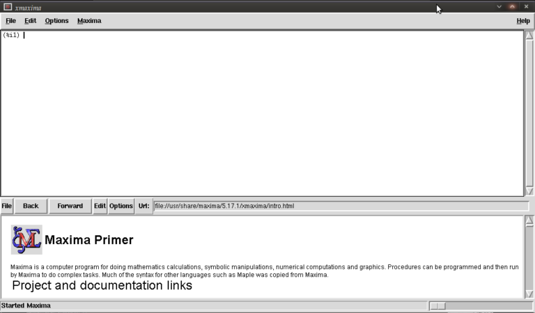
You are meant to type in the top most window next to (%i1) (input 1)
We first have to load the plotdf package (it isn’t loaded by default) so type:
load("plotdf");
and then press return (don’t forget the semi-colon or else nothing will happen (apart from a new line!)). it should respond with something similar to:
(%i1)  load("plotdf");
(%o1)  /usr/share/maxima/5.17.1/share/dynamics/plotdf.lisp
(%i2)
We will now race ahead and do our first plot. Keeping things simple for now we’ll do a phase plane plot for dx/dt = y, dy/dt = x, type:
plotdf([y,x]);
you should see something like this:
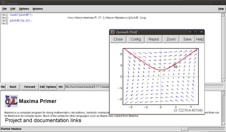
This is the Openmath plot window, (there are other plotting environments like Gnuplot but this function works only with Openmath) Notice that my pointer is directly below a red trajectory. These plots are interactive, you can draw other trajectories by clicking elsewhere. Try this. Hit the “replot” button and it will redraw the direction field with just your last trajectory.
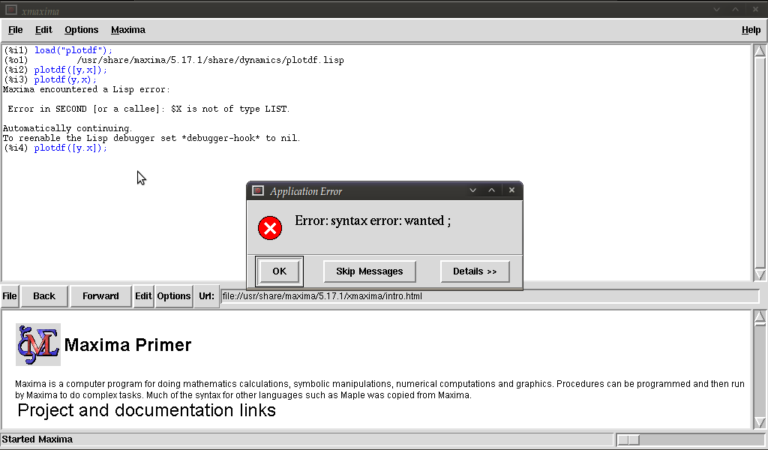
Before exploring any other options I want to purposely type some bad input and show how to fix things when it throws an error or gets stuck. Type
plotdf(y,x);
it should return
(%i3) plotdf(x,y);
Maxima encountered a Lisp error:

Error in SECOND [or a callee]: $Y is not of type LIST.

Automatically continuing.
To enable the Lisp debugger set *debugger-hook* to nil.
(%i4)
We forgot to put our functions for dx/dt,dy/dt in a list (square brackets). This is a reasonably safe error in that it tells us it isn’t happy and lets us continue.
Now type
plotdf([x.y]);
you should see something similar to
The problem this time was that we typed a dot instead of a comma (easily done), but worryingly when we close this message box and the blank plot the program will not process any commands. This can be fixed by clicking on the following in the xmaxima menu
file >> interrupt
where after telling you it encountered an error it should allow you to continue. One more; type
plotdf([2y,x]);
It should return with
  (%i5) plotdf([2y,x]);
  Incorrect syntax: Y is not an infix operator
  plotdf([2y,
           ^
  (%i5)
This time we forgot to put a binary operation such as * or + between 2 and y. If you come up with any other errors and the interrupt command is of no use you can still partially salvage things via
file >> restart
but you will, in this case, have to load plotdf again. (mercifully you can go to the line where you first typed it and press return (as with other commands you might have done))
I will now demonstrate some more “contrived” plots (for absolutely no purpose other than to shamelessly give a (very) small gallery of standard functions/operations etc… for the novice user) there is no need to type the last four unless you want to see what happens by changing constants/parameters, they’re the same plot :)
  plotdf([2*y-%e^(3/2)+cos((%pi/2)*x),log(abs(x))-%i^2*y]);
  plotdf([integrate(2*y,y)/y,diff((1/2)*x^2,x)]);
  plotdf([(3/%pi)*acos(1/2)*y,(2/sqrt(%pi))*x*integrate(exp(-x^2),x,0,inf)]);
  plotdf([floor(1.43)*y,ceiling(.35)*x]);
  plotdf([imagpart(x+%i*y),(sum(x^n,n,0,2)-sum(x^j,j,0,1))/x]);
I could go on…notice that the constants pi, e, and i are preceded by “%”. This tells maxima that they are known constants as opposed to symbols you happened to call “pi”, “e”, and “i”. Also, noting that the default range for x and y is (-10,10) in both cases; feel free to replot the first of those five without wrapping x inside “abs()” (inside the logarithm that is). remember file >> interrupt afterwards!
Now I will introduce you to some more of the parameters you can plug into “plotdf(…)”. close any plot windows and type
plotdf([x,y],[x,1,5],[y,-5,5]);
You should notice that x now ranges from 1 to 5, whilst y ranges from -5 to 5. There is nothing special about these numbers, we could have chosen any *real* numbers we liked. You can also use different symbols for your variables instead of x or y. Try
plotdf([v,u],[u,v]);
Note that I’ve declared u and v as variables in the second list. I will now purposely do something wrong again. Assign the value 5 to x by typing
x:5;
then type
plotdf([y,x]);
This time maxima won’t throw an error because syntactically you haven’t done anything wrong, you merely told it to do
plotdf([y,5]);
as opposed to what you really wanted which is
plotdf([y,x]);
Surprisingly to me (discovered as I’m writing this), changing the names of your variables like we did above won’t save you since it seems to treat new symbols as merely placeholders for it’s favourite symbols x and y. To get round this type
kill(x);
and this will put x back to what it originally was (the symbol x as opposed to 5).
You don’t actually have to provide expressions for dx/dt and dy/dt, you might instead know dy/dx and you can generate phaseplots by typing say
plotdf([x/y]);
In this case we didn’t actually need the square brackets because we are providing only one parameter: dy/dx (x will be set to t by maxima giving dx/dt = 1, and dy/dt = dy/dx = x/y)
A number of parameters can be changed from within the openmath window. Type
plotdf([y,x],[trajectory_at,-1,-2],[direction,forward]);
and then go into config. The screen you get should look something like this:
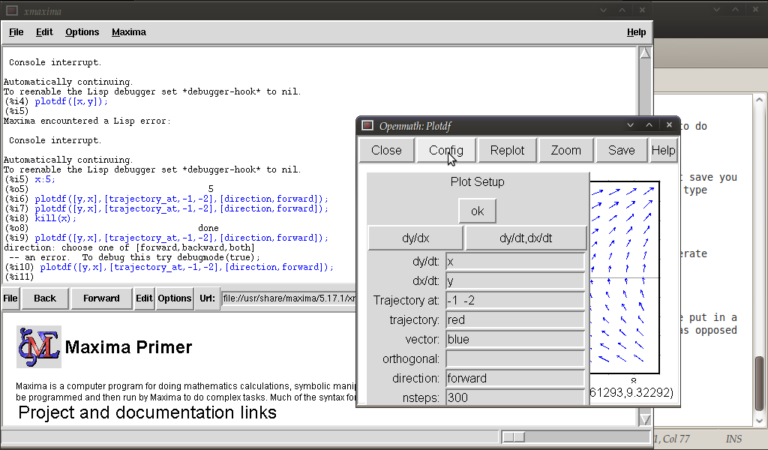
from here you can change the expressions for dx/dt, dy/dt, dy/dx, you can change colours and directions of trajectories (choices of forward, backward, both), change colours for direction arrows and orthogonal curves, starting points for trajectories (the two numbers separated by a space here, not a comma), time increments for t, number of steps used to create an integral curve. You can also look at an integral plots for x(t) and y(t) corresponding to the starting point given (or clicked) by hitting the “plot vs t” button. You can also zoom in or out by hitting the “zoom” button and clicking (or shift+clicking to unzoom), doing something else like hitting the config button will allow you to quit being in zoom mode click for trajectories again. (there might be a better way of doing this btw) You can also save these plots as eps files (you can then tweak these in other vector graphics based programs like Inkscape (free) or Adobe Illustrator etc..)
Interactive sliders
There are many permutations of things you can do (and you will surely find some of these by having a play) but my particular favourite is the option to use sliders allowing you to vary a parameter interactively and seeing what happens to the trajectories without constant replotting. ie:
plotdf([a*y,b*x],[sliders,"a=-1:3,b=-1:3"]);
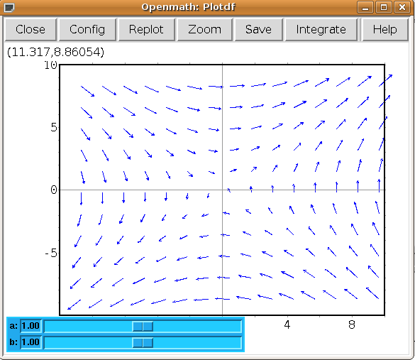
Hopefully, this has been enough to get people started, and for what it’s worth, the help file (though using xmaxima, you’ll find this in the web-browser version) for this topic has a pretty good gallery of different plots and other parameters I didn’t mention.
just to throw in one last thing in the spirit of experimentation, is the following set of commands:
A:matrix([0,1],[1,0]);
B:matrix([x],[y]);
plotdf([A[1].B,A[2].B);
which is another way of doing the same old
plotdf([y,x]);
where here I’ve made a 2×2 matrix A, a 2×1 matrix B, with A[1], A[2] denoting rows 1 and 2 of A respectively and matrix multiplied the rows of A by B (using A[1].B, A[2].B) to serve as inputs for dx/dt and dy/dt
Tutorial written by Gregory Astley, Mathematics Undergraduate at The University of Manchester.