
Archive for the ‘R’ Category
Update
A discussion on twitter determined that this was an issue with Locales. The practical upshot is that we can make R act the same way as the others by doing
Sys.setlocale("LC_COLLATE", "C")which may or may not be what you should do!
Original post
While working on a project that involves using multiple languages, I noticed some tests failing in one language and not the other. Further investigation revealed that this was essentially because R's default sort order for strings is different from everyone else's.
I have no idea how to say to R 'Use the sort order that everyone else is using'. Suggestions welcomed.
R 3.3.2
sort(c("#b","-b","-a","#a","a","b"))

[1] "-a" "-b" "#a" "#b" "a" "b"
Python 3.6
sorted({"#b","-b","-a","#a","a","b"})

['#a', '#b', '-a', '-b', 'a', 'b']
MATLAB 2018a
sort([{'#b'},{'-b'},{'-a'},{'#a'},{'a'},{'b'}])

ans =
1×6 cell array
{'#a'} {'#b'} {'-a'} {'-b'} {'a'} {'b'}
C++
int main(){

std::string mystrs[] = {"#b","-b","-a","#a","a","b"};
std::vector<std::string> stringarray(mystrs,mystrs+6);
std::vector<std::string>::iterator it;

std::sort(stringarray.begin(),stringarray.end());

for(it=stringarray.begin(); it!=stringarray.end();++it) {
   std::cout << *it << " ";
}

return 0;
}
Result:
#a #b -a -b a b
I’m working on optimising some R code written by a researcher at University of Sheffield and its very much a war of attrition! There’s no easily optimisable hotspot and there’s no obvious way to leverage parallelism. Progress is being made by steadily identifying places here and there where we can do a little better. 10% here and 20% there can eventually add up to something worth shouting about.
One such micro-optimisation we discovered involved multiplying two matrices together where one of them needed to be transposed. Here’s a minimal example.
#Set random seed for reproducibility
set.seed(3)

# Generate two random n by n matrices
n = 10
a = matrix(runif(n*n,0,1),n,n)
b = matrix(runif(n*n,0,1),n,n)

# Multiply the matrix a by the transpose of b
c = a %*% t(b)
When the speed of linear algebra computations are an issue in R, it makes sense to use a version that is linked to a fast implementation of BLAS and LAPACK and we are already doing that on our HPC system.
Here, I am using version 3.3.3 of Microsoft R Open which links to Intel’s MKL (an implementation of BLAS and LAPACK) on a Windows laptop.
In R, there is another way to do the computation c = a %*% t(b) — we can make use of the tcrossprod function (There is also a crossprod function for when you want to do t(a) %*% b)
c_new = tcrossprod(a,b)
Let’s check for equality
c_new == c
[,1] [,2] [,3] [,4] [,5] [,6] [,7] [,8] [,9] [,10]
[1,] TRUE TRUE TRUE TRUE TRUE TRUE TRUE TRUE TRUE TRUE
[2,] TRUE TRUE TRUE TRUE TRUE TRUE TRUE TRUE TRUE TRUE
[3,] TRUE TRUE TRUE TRUE TRUE TRUE TRUE TRUE TRUE TRUE
[4,] TRUE TRUE TRUE TRUE TRUE TRUE TRUE TRUE TRUE TRUE
[5,] TRUE TRUE TRUE TRUE TRUE TRUE TRUE TRUE TRUE TRUE
[6,] TRUE TRUE TRUE TRUE TRUE TRUE TRUE TRUE TRUE TRUE
[7,] TRUE TRUE TRUE TRUE TRUE TRUE TRUE TRUE TRUE TRUE
[8,] TRUE TRUE TRUE TRUE TRUE TRUE TRUE TRUE TRUE TRUE
[9,] TRUE TRUE TRUE TRUE TRUE TRUE TRUE TRUE TRUE TRUE
[10,] TRUE TRUE TRUE TRUE TRUE TRUE TRUE TRUE TRUE TRUE
Sometimes, when comparing the two methods you may find that some of those entries are FALSE which may worry you!
If that happens, computing the difference between the two results should convince you that all is OK and that the differences are just because of numerical noise. This happens sometimes when dealing with floating point arithmetic (For example, see https://www.walkingrandomly.com/?p=5380).
Let’s time the two methods using the microbenchmark package.
install.packages('microbenchmark')
library(microbenchmark)
We time just the matrix multiplication part of the code above:
microbenchmark(
original = a %*% t(b),
tcrossprod = tcrossprod(a,b)
)


Unit: nanoseconds
expr min lq mean median uq max neval
original 2918 3283 3491.312 3283 3647 18599 1000
tcrossprod 365 730 756.278 730 730 10576 1000
We are only saving microseconds here but that’s more than a factor of 4 speed-up in this small matrix case. If that computation is being performed a lot in a tight loop (and for our real application, it was), it can add up to quite a difference.
As the matrices get bigger, the speed-benefit in percentage terms gets lower but tcrossprod always seems to be the faster method. For example, here are the results for 1000 x 1000 matrices
#Set random seed for reproducibility
set.seed(3)

# Generate two random n by n matrices
n = 1000
a = matrix(runif(n*n,0,1),n,n)
b = matrix(runif(n*n,0,1),n,n)

microbenchmark(
original = a %*% t(b),
tcrossprod = tcrossprod(a,b)
)

Unit: milliseconds
expr min lq mean median uq max neval
original 18.93015 26.65027 31.55521 29.17599 31.90593 71.95318 100
tcrossprod 13.27372 18.76386 24.12531 21.68015 23.71739 61.65373 100
The cost of not using an optimised version of BLAS and LAPACK
While writing this blog post, I accidentally used the CRAN version of R. The recently released version 3.4. Unlike Microsoft R Open, this is not linked to the Intel MKL and so matrix multiplication is rather slower.
For our original 10 x 10 matrix example we have:
library(microbenchmark)
#Set random seed for reproducibility
set.seed(3)

# Generate two random n by n matrices
n = 10
a = matrix(runif(n*n,0,1),n,n)
b = matrix(runif(n*n,0,1),n,n)

microbenchmark(
original = a %*% t(b),
tcrossprod = tcrossprod(a,b)
)

Unit: microseconds
       expr   min    lq    mean median     uq    max neval
   original 3.647 3.648 4.22727  4.012 4.1945 22.611   100
 tcrossprod 1.094 1.459 1.52494  1.459 1.4600  3.282   100
Everything is a little slower as you might expect and the conclusion of this article — tcrossprod(a,b) is faster than a %*% t(b) — seems to still be valid.
However, when we move to 1000 x 1000 matrices, this changes
library(microbenchmark)
#Set random seed for reproducibility
set.seed(3)

# Generate two random n by n matrices
n = 1000
a = matrix(runif(n*n,0,1),n,n)
b = matrix(runif(n*n,0,1),n,n)

microbenchmark(
original = a %*% t(b),
tcrossprod = tcrossprod(a,b)
)

Unit: milliseconds
       expr      min       lq     mean   median       uq       max neval
   original 546.6008 587.1680 634.7154 602.6745 658.2387  957.5995   100
 tcrossprod 560.4784 614.9787 658.3069 634.7664 685.8005 1013.2289   100
As expected, both results are much slower than when using the Intel MKL-lined version of R (~600 milliseconds vs ~31 milliseconds) — nothing new there. More disappointingly, however, is that now tcrossprod is slightly slower than explicitly taking the transpose.
As such, this particular micro-optimisation might not be as effective as we might like for all versions of R.
I was recently invited to give a talk at the Sheffield R Users Group and decided to give a brief overview of how R relates to other technologies. Subjects included Mathematica’s integration of R, Intel’s compilers, Math Kernel Library and how they can make R faster and a range of Microsoft technologies including R Tools for Visual Studio, Microsoft R Open and the MRAN for reproducibility. I also touched upon the NAG Library, Maple’s code generation for R, GPUs and Spark.
- Slide deck: _ and R: How R relates to other technologies
Did I miss anything? If you were to give a similar talk, what might you have included?
I’ve just delivered a session called ‘R awareness’ to a group of IT staff at University of Manchester. The audience was a combination of desktop support, applications support and research software engineers and initial feedback indicates that it was well received.
The focus of the session was not the language itself but the software infrastructure that surrounds it. Multiple versions of R, packages, R Studio, Jupyter notebook, Microsoft R Open, SageMathCloud and the way that various applications such as Mathematica, Maple and Visual Studio interact with R.
I chose to deliver the material in the same way that The Code Cafe is delivered – self directed material where I act as facilitator. This seemed to work really well and there was a lot of conversation and interaction with the audience that I find is missing when doing a more traditional presentation.
Course material is at https://github.com/mikecroucher/R_awareness
A couple of weeks ago, a small group of us hit on the idea of running research programming tutorials in a cafe. The ‘plan’ was that we’d develop some self-paced programming tutorial material, take over a section of the main campus Cafe (Coffee Revolution) for a couple of hours in the evening and invite some researchers to come and learn something new for free.
For our first session, we chose to do a very gentle introduction to R. The students worked through the material, which started right at the beginning with installing R and RStudio, while a group of volunteer facilitators walked the room answering questions, solving problems and forming collaborations.

I can’t stress the importance of the facilitators enough! There is no chance that this format would have worked well without a group of skilled facilitators. On the day, I was joined by
- Research Software Engineer, David Jones
- PhD Student, Claire Green
- Post Doc, Will Furnass
I also had support of a few other people in the development stages. Thanks so much to all!
It was a lot of fun to do and student feedback has been fantastic! My favourite comment came from a medical doctor who said ‘I had no idea about computer programming and I don’t think I would be brave enough to try it on my own. Yesterday, I realised that R can be something useful and not really hard to learn.’
I find interactions like this to be hugely motivational!
There was a real buzz in the room, everyone seemed to learn something useful and I walked away from the evening with a couple of interesting follow-up collaborations in the bag. There were lots of calls for future sessions on topics ranging from more advanced R through to Python, MATLAB, Mathematica and High Performance Computing. The self-paced, flipped-classroom style of teaching was also a great hit!
So, that’s what went right. What about what went wrong?
Installation Problems
We deliberately allowed time for the installation of R in the session. Ensuring that the attendees had a working install of R and RStudio on their own kit was part of the point. Before the session, I did trial installs on Windows and Mac and everything went without a hitch. Other members of the team tried fresh installs on Linux.
“Installation’s going to be a doddle…no worries” I thought.
The very first attendee who called me over for help couldn’t get RStudio started on her Mac. It crapped out with an error message I’d never seen before. A bit of googling determined that it was because she had several old versions of R already installed and RStudio took exception to this.
We also had Linux users of various flavours and most of them had problems. A user of Arch Linux gave up on trying to install RStudio and used the command line instead. One linux user called me over after he started installing the ggplot2 package asking ‘This has been compiling for ages, is that normal?’ Fortunately, we were in a cafe so he could go get himself a brew while waiting.
Some people already had versions of R and RStudio installed from waaaaay back and so didn’t feel it necessary to upgrade to the latest versions. These people discovered that they couldn’t install packages because ‘foo isn’t available for R version whatever’.
It was all rather painful to be honest! We were in full technical-support mode…but at least people left the session with working, up to date versions R and R Studio….mostly!
Power!
There wen’t many power sockets. We didn’t think much about this in advance. Ball dropped!
For a feeble attempt at a defence I’ll mention that the battery on my laptop is superb and I spend hours working in the host cafe without worrying about power. Since I’ve been so spoiled, I’ve forgotten how important a mains socket is when your battery sucks.
Next Steps
This session was an experiment — something quickly spun up to see if it might work. I’m happy to report that it did!
Our main problem is that we’ve now created demand. Demand for repeats of this session for new audiences, demand for new material and demand for further consultancy. How fortunate for us at Sheffield that we have a newly created Research Software Engineering group to help meet this demand.
Say you have two vectors in R (These are taken from my tutorial Simple nonlinear least squares curve fitting in R)
xdata = c(-2,-1.64,-1.33,-0.7,0,0.45,1.2,1.64,2.32,2.9)
ydata = c(0.699369,0.700462,0.695354,1.03905,1.97389,2.41143,1.91091,0.919576,-0.730975,-1.42001)
We put these in a data frame with
data = data.frame(xdata=xdata,ydata=ydata)
This looks like this in R
   xdata     ydata
1  -2.00  0.699369
2  -1.64  0.700462
3  -1.33  0.695354
4  -0.70  1.039050
5   0.00  1.973890
6   0.45  2.411430
7   1.20  1.910910
8   1.64  0.919576
9   2.32 -0.730975
10  2.90 -1.420010
Exporting to a .csv file is done using the standard R function, write.csv
write.csv(data,file='example_data.csv')
The resulting .csv file looks like this:
"","xdata","ydata"
"1",-2,0.699369
"2",-1.64,0.700462
"3",-1.33,0.695354
"4",-0.7,1.03905
"5",0,1.97389
"6",0.45,2.41143
"7",1.2,1.91091
"8",1.64,0.919576
"9",2.32,-0.730975
"10",2.9,-1.42001
I don’t want to include the row numbers in my output. To achieve this, we do
write.csv(data,file='example_data.csv',row.names=FALSE)
This gets us a file that looks like this:
 "xdata","ydata"
-2,0.699369
-1.64,0.700462
-1.33,0.695354
-0.7,1.03905
0,1.97389
0.45,2.41143
1.2,1.91091
1.64,0.919576
2.32,-0.730975
2.9,-1.42001
I can also remove the quotes around xdata and ydata with quote=FALSE
write.csv(data,file='example_data.csv',row.names=FALSE,quote=FALSE)
giving the file below
xdata,ydata
-2,0.699369
-1.64,0.700462
-1.33,0.695354
-0.7,1.03905
0,1.97389
0.45,2.41143
1.2,1.91091
1.64,0.919576
2.32,-0.730975
2.9,-1.42001
Changing the separator
Despite the fact that they are asking R to write a comma separated file, some people try to change the separator. Perhaps you’d like to try changing it to a tab for example. The following looks reasonable:
write.csv(data,file='example_data.csv',row.names=FALSE,quote=FALSE,sep="\t")
Although it understands what you are trying to do, R will completely ignore your request!
Warning message:
In write.csv(data, file = "example_data.csv", row.names = FALSE,  :
  attempt to set 'sep' ignored
This is because write.csv is designed to ensure that some standard .csv conventions are followed. It’s trying to protect you against yourself!
In the UK, the convention for .csv files is to use . for a decimal point and , as a separator and that’s the convention that write.csv sticks to. Other countries have a different convention – they use a , for the decimal point and a ; for the separator. The function write.csv2 takes care of that for you.
If you absolutely must change the separator to something else, make use of write.table instead:
write.table(data,file='example_data.csv',row.names=FALSE,quote=FALSE,sep="\t")
Now, the file will come out like this:
xdata   ydata
-2      0.699369
-1.64   0.700462
-1.33   0.695354
-0.7    1.03905
0       1.97389
0.45    2.41143
1.2     1.91091
1.64    0.919576
2.32    -0.730975
2.9     -1.42001
Further reading: Official write.table documentation in R
While waiting for the rain to stop before heading home, I started messing around with the heart equation described in an old WalkingRandomly post. Playing code golf with myself, I worked to get the code tweetable. In Python:
from pylab import *
x=r_[-2:2:0.001]
show(plot((sqrt(cos(x))*cos(200*x)+sqrt(abs(x))-0.7)*(4-x*x)**0.01)) pic.twitter.com/gbOTbYSaIG— Mike Croucher (@walkingrandomly) February 8, 2016
In R:
x=seq(-2,2,0.001)
y=Re((sqrt(cos(x))*cos(200*x)+sqrt(abs(x))-0.7)*(4-x*x)^0.01)
plot(x,y)#rstats pic.twitter.com/trpgEnNna4— Mike Croucher (@walkingrandomly) February 8, 2016
I liked the look of the default plot in R so animated it by turning 200 into a parameter that ranged from 1 to 200. The result was this animation:
Finding this animation based on previous tweets oddly mesmerising #rstats pic.twitter.com/e3q6lZqWcP
— Mike Croucher (@walkingrandomly) February 8, 2016
The code for the above isn’t quite tweetable:
options(warn=-1)
for(num in seq(1,200,1))
{
    filename = paste("rplot" ,sprintf("%03d", num),'.jpg',sep='')
    jpeg(filename)
    x=seq(-2,2,0.001)
    y=Re((sqrt(cos(x))*cos(num*x)+sqrt(abs(x))-0.7)*(4-x*x)^0.01)
    plot(x,y,axes=FALSE,ann=FALSE)
    dev.off()
}
This produces a lot of .jpg files which I turned into the animated gif with ImageMagick:
convert -delay 12 -layers OptimizeTransparency -colors 8 -loop 0 *.jpg animated.gif
A recent trend on Facebook is to create a wordcloud of all of your posts using an external service. I chose not to use it because I tend to use Facebook for personal interactions among close friends and I didn’t want to send all of my data to another external company.
Twitter is a different matter, however! All of the data is open and it’s very easy to write a computer program to generate Twitter world clouds without the need for an external service.
I wrote a simple script in R that generates a wordcloud from the most recent 3200 tweets and outputs the top 200 words (get the code on github). The script removes many of the uninteresting words such as the, of, and that would otherwise dominate the cloud. These stopwords come from the Top100Words list of the R package qdap but I also added a few more such as ‘just’ and ‘me’ that I seem to use a lot.
This is the current wordcloud for my twitter account, walkingrandomly. Click on the image to see a bigger version. My main interests are very clear – Python programming, research software, data and anything that’s new!

Once I had seen my wordcloud, I wondered how things would look for other twitter users who I pay a lot of attention to. This is how it looks for Manchester University’s Nick Higham. Clearly he’s big on SIAM, Manchester, and Matrix Analysis!

I then looked at my manager at Sheffield University, Neil Lawrence. Neil finds data and the city of Sheffield very important and also writes about workshops, science, blog posts and machine learning a lot.

The R code that generated these wordclouds is available on github but it won’t work out of the box. You’ll need to register with twitter for app development (It’s free and fairly straightforward) and get various access keys before you can use the code.
I recently found myself in need of a portable install of the Jupyter notebook which made use of a portable install of R as the compute kernel. When you work in institutions that have locked-down managed Windows desktops, such portable installs can be a life-saver! This is particularly true when you are working with rapidly developing projects such as Jupyter and IRKernel.
It’s not perfect but it works for the fairly modest requirements I had for it. Here are the steps I took to get it working.
Download and install Portable Python
I downloaded Portable Python 2.7.6.1 from http://portablepython.com/ and installed into a directory called Portable Python 2.7.6.1
Update IPython and install the extra modules we need
This version of Portable Python comes with a portable IPython instance but it is too old to support alternative kernels. As such, we need to install a newer version.
Open a cmd.exe command prompt and navigate to Portable Python 2.7.6.1\App\Scripts.
Enter the command
easy_install ipython.exe
You’ll now find that you can launch the ipython.exe terminal from within this directory:
C:\Users\walkingrandomly\Desktop\Portable Python 2.7.6.1\App\Scripts>ipython
Python 2.7.6 (default, Nov 10 2013, 19:24:18) [MSC v.1500 32 bit (Intel)]
Type "copyright", "credits" or "license" for more information.

IPython 3.1.0 -- An enhanced Interactive Python.
?         -> Introduction and overview of IPython's features.
%quickref -> Quick reference.
help      -> Python's own help system.
object?   -> Details about 'object', use 'object??' for extra details.

In [1]: exit()
If you try to launch the notebook, however, you’ll get error messages. This is because we haven’t taken care of all the dependencies. Let’s do that now. Ensuring you are still in the Portable Python 2.7.6.1\App\Scripts folder, execute the following commands.
easy_install pyzmq
easy_install jinja2
easy_install tornado
easy_install jsonschema
You should now be able to launch the notebook using
ipython notebook
Install portable R and IRKernel
- I downloaded Portable R 3.2 from http://sourceforge.net/projects/rportable/files/ and installed into a directory called R-Portable
- Move this directory into the Portable Python directory. It needs to go inside Portable Python 2.7.6.1\App (see this discussion to learn how I discovered that this location was the correct one)
- Launch the Portable R executable which should be at Portable Python 2.7.6.1\App\R-Portable\R-portable.exe and install the IRKernel packages by doing
install.packages(c("rzmq","repr","IRkernel","IRdisplay"), repos="http://irkernel.github.io/")
Install additional R packages
The version of Portable R I used didn’t include various necessary packages. Here’s how I fixed that.
- Launch the Portable R executable which should be at Portable Python 2.7.6.1\App\R-Portable\R-portable.exe and install the following packages
install.packages('digest')
install.packages('uuid')
install.packages('base64enc')
install.packages('evaluate')
install.packages('jsonlite')
Install the R kernel file
Create the directory structure Portable Python 2.7.6.1\App\share\jupyter\kernels\R_kernel
Create a file called kernel.json that contains the following
{"argv": ["R-Portable/App/R-Portable/bin/i386/R.exe","-e","IRkernel::main()",
"--args","{connection_file}"],
 "display_name":"Portable R"
}
This file needs to go in the R_kernel directory created earlier. Note that the kernel location specified in kernel.json uses Linux style forward slashes in the path rather than the backslashes that Windows users are used to. I found that this was necessary for the kernel to work –it was ignored by the notebook otherwise.
Finishing off
Everything created so far, including R, is in the folder Portable Python 2.7.6
I created a folder called PortableJupyter and put the Portable Python 2.7.6 folder inside it. I also created the folder PortableJupyter\notebooks to allow me to carry my notebooks around with the software that runs them.
There is a bug in Portable Python 2.7.6.1 relating to scripts like IPython.exe that have been installed using easy_install. In short, they stop working if you move the directory they’re installed in – breaking portability somewhat! (Details here)
The workaround is to launch Ipython by running the script Portable Python 2.7.6.1\App\Scripts\ipython-script.py
I didn’t want to bother with that so created a shortcut in my PortableJupyter folder called Launch notebook. The target of this shortcut was the following line
%windir%\system32\cmd.exe /c "cd notebooks && "%CD%/Portable Python 2.7.6.1/App\python.exe" "%CD%/Portable Python 2.7.6.1\App\Scripts\ipython-script.py" notebook"
This starts the notebook using the default web browser and puts you in the notebooks directory.
The pay off
My folder looks like this:
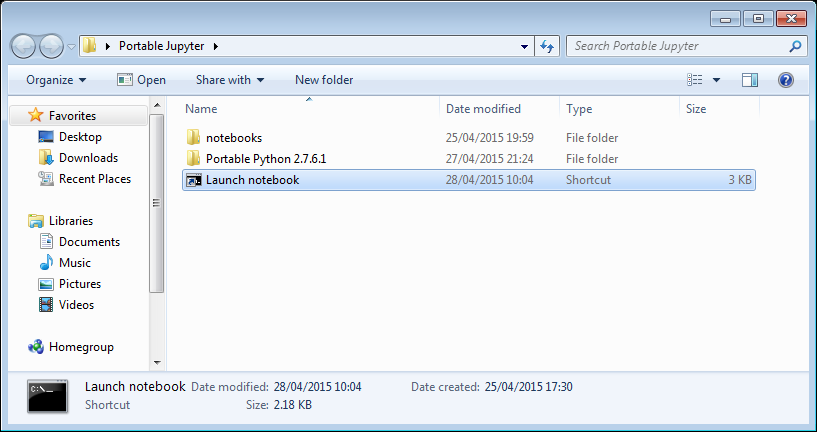
If I click on the Launch Notebook shortcut, I get a Jupyter session with 2 kernel options
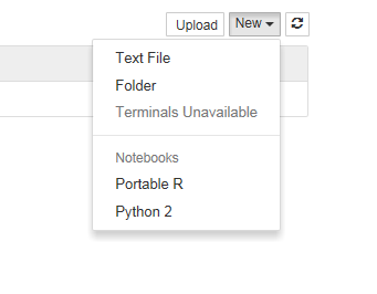
I can choose the Portable R kernel and start using R in the notebook!

RLink is Mathematica’s interface to the R language – a feature that has been extremely popular since its debut in Mathematica version 9. It’s a great package but has one or two issues. For example, RLink makes use of a built in version of R which is currently stuck at the rather old version 2.14. Official support for the use of external versions of R and adding third-party libraries varies by operating system and version of Mathematica. Windows support is great — OS X support, not so much.
Expert Mathematica user Szabolcs Horvát has written the definitive guide on how to get RLink up and running with the latest version of R on all three major operating systems, building on earlier work by Leonid Shifrin and members of the Mathematica Stack Exchange community. Thanks to this work, we can now enjoy any version of R we like with Mathematica!