
Archive for the ‘R’ Category
A colleague recently sent me the following code snippet in R
> a=c(1,2,3,40)
> b=a[1:10]
> b
[1]  1  2  3 40 NA NA NA NA NA NA
The fact that R didn’t issue a warning upset him since exceeding array bounds, as we did when we created b, is usually a programming error.
I’m less concerned and simply file the above away in an area of my memory entitled ‘Odd things to remember about R’ — I find that most programming languages have things that look odd when you encounter them for the first time. With that said, I am curious as to why the designers of R thought that the above behaviour was a good idea.
Does anyone have any insights here?
The R code used for this example comes from Barry Rowlingson, so huge thanks to him.
A question I get asked a lot is ‘How can I do nonlinear least squares curve fitting in X?’ where X might be MATLAB, Mathematica or a whole host of alternatives. Since this is such a common query, I thought I’d write up how to do it for a very simple problem in several systems that I’m interested in
This is the R version. For other versions,see the list below
- Simple nonlinear least squares curve fitting in Julia
- Simple nonlinear least squares curve fitting in Maple
- Simple nonlinear least squares curve fitting in Mathematica
- Simple nonlinear least squares curve fitting in MATLAB
- Simple nonlinear least squares curve fitting in Python
The problem
xdata = -2,-1.64,-1.33,-0.7,0,0.45,1.2,1.64,2.32,2.9
ydata = 0.699369,0.700462,0.695354,1.03905,1.97389,2.41143,1.91091,0.919576,-0.730975,-1.42001
and you’d like to fit the function

using nonlinear least squares. You’re starting guesses for the parameters are p1=1 and P2=0.2
For now, we are primarily interested in the following results:
- The fit parameters
- Sum of squared residuals
- Parameter confidence intervals
Future updates of these posts will show how to get other results. Let me know what you are most interested in.
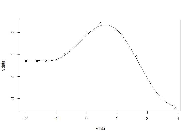
Solution in R
# construct the data vectors using c()
xdata = c(-2,-1.64,-1.33,-0.7,0,0.45,1.2,1.64,2.32,2.9)
ydata = c(0.699369,0.700462,0.695354,1.03905,1.97389,2.41143,1.91091,0.919576,-0.730975,-1.42001)

# look at it
plot(xdata,ydata)

# some starting values
p1 = 1
p2 = 0.2

# do the fit
fit = nls(ydata ~ p1*cos(p2*xdata) + p2*sin(p1*xdata), start=list(p1=p1,p2=p2))

# summarise
summary(fit)
This gives
Formula: ydata ~ p1 * cos(p2 * xdata) + p2 * sin(p1 * xdata)

Parameters:
   Estimate Std. Error t value Pr(>|t|)
p1 1.881851   0.027430   68.61 2.27e-12 ***
p2 0.700230   0.009153   76.51 9.50e-13 ***
---
Signif. codes:  0 ‘***’ 0.001 ‘**’ 0.01 ‘*’ 0.05 ‘.’ 0.1 ‘ ’ 1

Residual standard error: 0.08202 on 8 degrees of freedom

Number of iterations to convergence: 7
Achieved convergence tolerance: 2.189e-06
Draw the fit on the plot by getting the prediction from the fit at 200 x-coordinates across the range of xdata
new = data.frame(xdata = seq(min(xdata),max(xdata),len=200))
lines(new$xdata,predict(fit,newdata=new))
Getting the sum of squared residuals is easy enough:
sum(resid(fit)^2)
Which gives
[1] 0.0538127
Finally, lets get the parameter confidence intervals.
confint(fit)
Which gives
Waiting for profiling to be done...
        2.5%     97.5%
p1 1.8206081 1.9442365
p2 0.6794193 0.7209843
I was recently working with someone who was running thousands of R jobs on our Condor pool and some of them were failing. As part of the diagnostic process, we needed to determine which machines in the pool were causing the problem. My solution was to add the line
hostname
To the Bash script that eventually called R and the program he was running. This gives output that looks like this
badmachine.ourdomain.ac.uk
His solution was to do exactly the same thing in R. To do this, he added the following line to the beginning of his R script
(Sys.info()["nodename"])
Which produces output that looks like
nodename
"badmachine.ourdomain.ac.uk"
Either way, the job was done.
R has a citation() command that recommends how to cite the use of R in your publications, information that is also included in R’s Frequently Asked Questions document.
To cite R in publications use:

  R Core Team (2012). R: A language and environment for
  statistical computing. R Foundation for Statistical
  Computing, Vienna, Austria. ISBN 3-900051-07-0, URL
  http://www.R-project.org/.

A BibTeX entry for LaTeX users is

  @Manual{,
    title = {R: A Language and Environment for Statistical Computing},
    author = {{R Core Team}},
    organization = {R Foundation for Statistical Computing},
    address = {Vienna, Austria},
    year = {2012},
    note = {{ISBN} 3-900051-07-0},
    url = {http://www.R-project.org/},
  }

We have invested a lot of time and effort in creating R, please
cite it when using it for data analysis. See also
‘citation("pkgname")’ for citing R packages
This led me to wonder how often people cite the software they use. For example, if you publish the results of a simulation written in MATLAB do you cite MATLAB in any way? How about if you used Origin or Excel to produce a curve fit, would you cite that? Would you cite your plotting software, numerical libraries or even compiler?
The software sustainability institute (SSI), of which I recently became a fellow, has guidelines on how to cite software.
xkcd is a popular webcomic that sometimes includes hand drawn graphs in a distinctive style. Here’s a typical example

In a recent Mathematica StackExchange question, someone asked how such graphs could be automatically produced in Mathematica and code was quickly whipped up by the community. Since then, various individuals and communities have developed code to do the same thing in a range of languages. Here’s the list of examples I’ve found so far
- xkcd style graphs in Mathematica. There is also a Wolfram blog post on this subject.
- xkcd style graphs in R. A follow up blog post at vistat.
- xkcd style graphs in LaTeX
- xkcd style graphs in Python using matplotlib
- xkcd style graphs in MATLAB. There is now some code on the File Exchange that does this with your own plots.
- xkcd style graphs in javascript using D3
- xkcd style graphs in Euler
- xkcd style graphs in Fortran
Any I’ve missed?
My attention was recently drawn to a Google+ post by JerWei Zhang where he evaluates 2^3^4 in various packages and notes that they don’t always agree. For example, in MATLAB 2010a we have 2^3^4 = 4096 which is equivalent to putting (2^3)^4 whereas Mathematica 8 gives 2^3^4 = 2417851639229258349412352 which is the same as putting 2^(3^4). JerWei’s post gives many more examples including Excel, Python and Google and the result is always one of these two (although to varying degrees of precision).
What surprised me was the fact that they disagreed at all since I thought that the operator precendence rules were an agreed standard across all software packages. In this case I’d always use brackets since _I_ am not sure what the correct interpretation of 2^3^4 should be but I would have taken it for granted that there is a standard somewhere and that all of the big hitters in the numerical world would adhere to it.
Looks like I was wrong!
I was recently given the task of converting a small piece of code written in R, the free open-source programming language heavily used by statisticians, into MATLAB which was an interesting exercise since I had never coded a single line of R in my life! Fortunately for me, the code was rather simple and I didn’t have too much trouble with it but other people may not be so lucky since both MATLAB and R can be rather complicated to say the least. Wouldn’t it be nice if there was a sort of Rosetta Stone that helped you to translate between the two systems?
Happily, it turns out that there is in the form of The MATLAB / R Reference by David Hiebeler which gives both the R and MATLAB commands for hundreds of common (and some not so common) operations.
While flicking through the 47 page document I noted that there are a few MATLAB commands for which David hasn’t found an R equivalent (possibly because there simply isn’t one of course). For example, at number 161 of David’s document he describes the MATLAB command
yy=spline(x,y,xx)
which he describes as
‘Fit cubic spline with “not-a-knot” conditions (the first two piecewise cubics coincide,as do the last two), to points (xi , yi ) whose coordinates are in vectors x and y; evaluate at points whose x coordinates are in vector xx, storing corresponding y’s in yy.’
At the moment David doesn’t know of an R equivalent so if you are a R master then maybe you could help out with this extremely useful document?