
Archive for the ‘GPU’ Category
Just over 4 years ago I was very happy with the 1.2 Teraflops of single precision performance I measured on my then-new Dell XPS 95600 laptop using MATLAB’s GPU Bench and noted that its performance was on-par with the first supercomputer I supported professionally. Double precision performance stank of course but I had gotten used to that with laptop GPUs!
Fast forward to 2021 and my personal computational landscape has changed substantially. The pandemic has confined me to my home office and high performance laptops don’t have quite the same allure that they did when I was doing most of my interesting computational work in airports and coffee shops. I swapped a 15 inch screen for a 49 inch Ultrawide monitor and my laptop is gathering dust while I enjoy my new Dell desktop with an 8 core Intel i7-11700 and an NVIDIA GTX 3070.
This is the first desktop machine I’ve personally owned for almost two decades and the amount of performance I got for less money than the high spec laptops I used to favour is astonishing! Here are the GPU Bench results using MATLAB 2021a
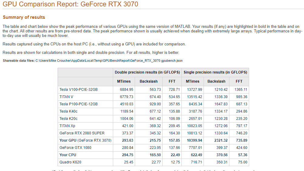
The standout figure is 10,399 Gigaflops for single precision Matrix-Matrix multiplication. At only slightly shy of 10.4 Teraflops that’s almost an order of magnitude faster than the results that impressed me on my laptop 4 years ago!
Double precision performance is nothing to write home about but it never is on consumer NVIDIA GPU cards. I stopped being upset about that years ago!
The other result I find interesting with respect to my personal history of devices is the 622 Gigaflops result for single precision from the Intel i7 CPU. This is getting on for twice as fast as the GPU on my 2015 Apple MacbookPro which managed 349 Gigaflops….a machine I still use today although primarily for Netflix.
My friends over at the University of Sheffield Research Software Engineering group are running a GPU Hackathon sponsored by Nvidia. The event will be on August 19-23 2019 in Sheffield, United Kingdom. The call for proposals is at http://gpuhack.shef.ac.uk/
The Sheffield team have this to say about the event:
We are looking for teams of 3-5 developers with a scalable** application to port to or optimize on a GPU accelerator. Collectively the team must have complete knowledge of the application. If the application is a suite of apps, no more than two per team will be allowed and a minimum of 2 people per app must attend. Space will be limited to 8 teams.
** By scalable we mean node-to-node communication implemented, but don’t be discouraged from applying if your application is less than scalable. We are also looking for breadth of application areas.
The goal of the GPU hackathon is for current or prospective user groups of large hybrid CPU-GPU systems to send teams of at least 3 developers along with either:
- (potentially) scalable application that could benefit from GPU accelerators, or
- An application running on accelerators that needs optimization.
There will be intensive mentoring during this 5-day hands-on workshop, with the goal that the teams leave with applications running on GPUs, or at least with a clear roadmap of how to get there.
My new toy is a 2017 Dell XPS 15 9560 laptop on which I am running Windows 10. Once I got over (and fixed) the annoyance of all the advertising in Windows Home, I quickly starting loving this new device.
To get a handle on its performance, I used GPUBench in MATLAB 2016b and got the following results (This was the best of 4 runs…I note that MTimes performance for the CPU (Host PC), for example, varied between 130 and 150 Glops).
- CPU: Intel Core I7-7700HQ (6M Cache, up to 3.8Ghz)
- GPU: NVIDIA GTX 1050 with 4GB GDDR5
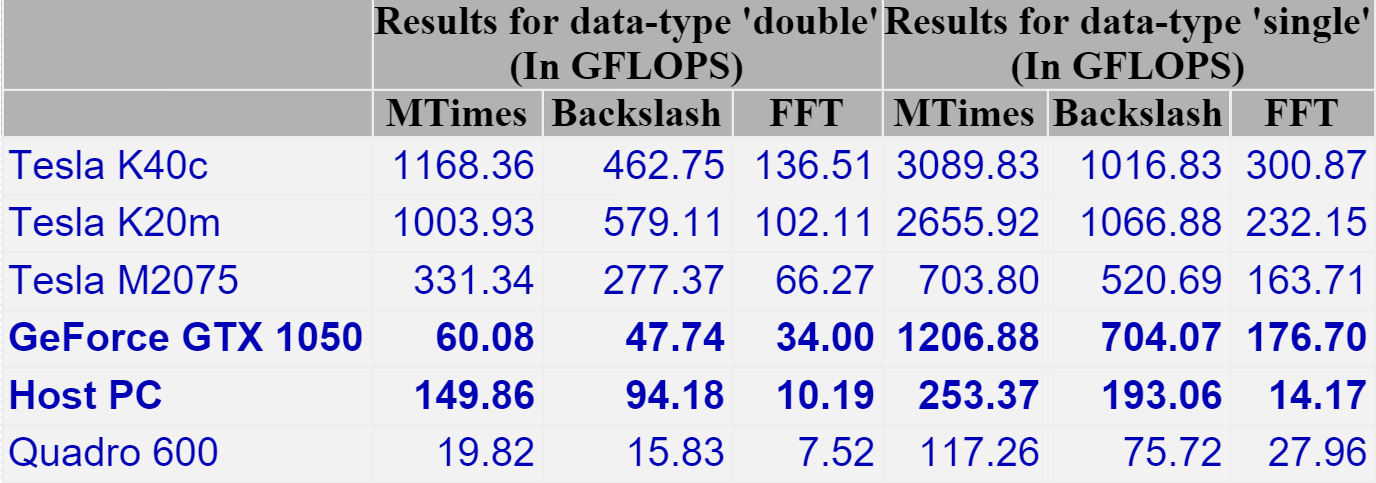
I last did this for my Retina MacBook Pro and am happy to see that the numbers are better across the board. The standout figure for me is the 1206 Gflops (That’s 1.2 Teraflops!) of single precision performance for Matrix-Matrix Multiply.
That figure of 1.2 Teraflops rang a bell for me and it took me a while to realise why…..
My laptop vs Manchester University’s old HPC system – Horace
Old timers like me (I’m almost 40) like to compare modern hardware with bygone supercomputers (1980s Crays vs mobile phones for example) and we know we are truly old when the numbers coming out of laptop benchmarks match the peak theoretical performance of institutional HPC systems we actually used as part of our career.
This has now finally happened to me! I was at the University of Manchester when it commissioned a HPC service called Horace and I was there when it was switched off in 2010 (only 6 and a bit years ago!). It was the University’s primary HPC service with a support team, helpdesk, sysadmins…the lot. The specs are still available on Manchester’s website:
- 24 nodes, each with 8 cores giving 192 cores in total.
- Each core had a theoretical peak compute performance of 6.4 double precision Gflop/s
- So a node had a theoretical peak performance of 51.2 Gflop/s
- The whole thing could theoretically manage 1.2 Teraflop/s
- It had four special ‘high memory’ nodes with 32Gb RAM each
Good luck getting that 1.2 Teraflops out of it in practice!
I get a big geek-kick out of the fact that my new laptop has the same amount of RAM as one of these ‘big memory’ nodes and that my laptop’s double precision CPU performance is on par with the combined power of 3 of Horace’s nodes. Furthermore, my laptop’s GPU can just about manage 1.2 Teraflop/s of single precision performance in MATLAB — on par with the total combined power of the HPC system*.
* (I know, I know….Horace’s numbers are for double precision and my GPU numbers are single precision — apples to oranges — but it still astonishes me that the headline numbers are the same — 1.2 Teraflops).
I recently got a 15 inch Retina Macbook Pro which contains an NVIDIA GT 750M GPU. It’s been a while since I last got a laptop with a decent GPU in it so I wondered how it would perform in MATLAB using the Parallel Computing Toolbox.
Of course I didn’t read any documentation; I simply fired up MATLAB 2015a and issued the gpuDevice command.
>> gpuDevice
Error using gpuDevice (line 26)
There is a problem with the CUDA driver or with this GPU device. Be sure
that you have a supported GPU and that the latest driver is installed.

Caused by:
    The CUDA driver could not be loaded. The library name used was
    '/usr/local/cuda/lib/libcuda.dylib'. The error was:
    dlopen(/usr/local/cuda/lib/libcuda.dylib, 10): image not found
This is because I didn’t install a load of CUDA-related stuff! Following these instructions did the trick!
>> gpuDevice()

ans =

  CUDADevice with properties:

                      Name: 'GeForce GT 750M'
                     Index: 1
         ComputeCapability: '3.0'
            SupportsDouble: 1
             DriverVersion: 6.5000
            ToolkitVersion: 6.5000
        MaxThreadsPerBlock: 1024
          MaxShmemPerBlock: 49152
        MaxThreadBlockSize: [1024 1024 64]
               MaxGridSize: [2.1475e+09 65535 65535]
                 SIMDWidth: 32
               TotalMemory: 2.1470e+09
           AvailableMemory: 444055552
       MultiprocessorCount: 2
              ClockRateKHz: 925500
               ComputeMode: 'Default'
      GPUOverlapsTransfers: 1
    KernelExecutionTimeout: 1
          CanMapHostMemory: 1
           DeviceSupported: 1
            DeviceSelected: 1
I headed over to the MATLAB File Exchange to get the GPU Bench App for MATLAB and fired it up. The summary of the results is below. Click on the image to see the detailed results.
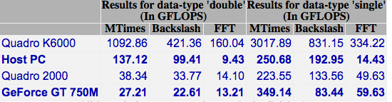
The double precision performance of this GPU card is very poor – MUCH slower than the CPU on the Macbook Pro.
Looking on the bright side, the numbers for the CPU are pretty good for a laptop!
One of my academic colleagues, Fumie Costen, recently asked members of The University of Manchester GPU Club the following question
‘I am looking for a journal with high impact factor where I can publish our work on GPU for FDTD computations. Can anyone help?’
So far, we haven’t had any replies so I’m throwing the question open to the world. Any suggestions?
Ever since I took a look at GPU accelerating simple Monte Carlo Simulations using MATLAB, I’ve been disappointed with the performance of its GPU random number generator. In MATLAB 2012a, for example, it’s not much faster than the CPU implementation on my GPU hardware. Consider the following code
function gpuRandTest2012a(n)

mydev=gpuDevice();
disp('CPU - Mersenne Twister');
tic
CPU = rand(n);
toc

sg = parallel.gpu.RandStream('mrg32k3a','Seed',1);
parallel.gpu.RandStream.setGlobalStream(sg);
disp('GPU - mrg32k3a');
tic
Rg = parallel.gpu.GPUArray.rand(n);
wait(mydev);
toc
Running this on MATLAB 2012a on my laptop gives me the following typical times (If you try this out yourself, the first run will always be slower for various reasons I’ll not go into here)
>> gpuRandTest2012a(10000)
CPU - Mersenne Twister
Elapsed time is 1.330505 seconds.
GPU - mrg32k3a
Elapsed time is 1.006842 seconds.
Running the same code on MATLAB 2012b, however, gives a very pleasant surprise with typical run times looking like this
CPU - Mersenne Twister
Elapsed time is 1.590764 seconds.
GPU - mrg32k3a
Elapsed time is 0.185686 seconds.
So, generation of random numbers using the GPU is now over 7 times faster than CPU generation on my laptop hardware–a significant improvment on the previous implementation.
New generators in 2012b
The MATLAB developers went a little further in 2012b though. Not only have they significantly improved performance of the mrg32k3a combined multiple recursive generator, they have also implemented two new GPU random number generators based on the Random123 library. Here are the timings for the generation of 100 million random numbers in MATLAB 2012b
- Get the code – gpuRandTest2012b.m
CPU - Mersenne Twister
Elapsed time is 1.370252 seconds.
GPU - mrg32k3a
Elapsed time is 0.186152 seconds.
GPU - Threefry4x64-20
Elapsed time is 0.145144 seconds.
GPU - Philox4x32-10
Elapsed time is 0.129030 seconds.
Bear in mind that I am running this on the relatively weak GPU of my laptop! If anyone runs it on something stronger, I’d love to hear of your results.
- Laptop model: Dell XPS L702X
- CPU: Intel Core i7-2630QM @2Ghz software overclockable to 2.9Ghz. 4 physical cores but total 8 virtual cores due to Hyperthreading.
- GPU: GeForce GT 555M with 144 CUDA Cores. Graphics clock: 590Mhz. Processor Clock:1180 Mhz. 3072 Mb DDR3 Memeory
- RAM: 8 Gb
- OS: Windows 7 Home Premium 64 bit.
- MATLAB: 2012a/2012b
Intel have finally released the Xeon Phi – an accelerator card based on 60 or so customised Intel cores to give around a Teraflop of double precision performance. That’s comparable to the latest cards from NVIDIA (1.3 Teraflops according to http://www.theregister.co.uk/2012/11/12/nvidia_tesla_k20_k20x_gpu_coprocessors/) but with one key difference—you don’t need to learn any new languages or technologies to take advantage of it (although you can do so if you wish)!
The Xeon Phi uses good, old fashioned High Performance Computing technologies that we’ve been using for years such as OpenMP and MPI. There’s no need to completely recode your algorithms in CUDA or OpenCL to get a performance boost…just a sprinkling of OpenMP pragmas might be enough in many cases. Obviously it will take quite a bit of work to squeeze every last drop of performance out of the thing but this might just be the realisation of ‘personal supercomputer’ we’ve all been waiting for.
Here are some links I’ve found so far — would love to see what everyone else has come up with. I’ll update as I find more
- http://www.theregister.co.uk/2012/11/12/intel_xeon_phi_coprocessor_launch/ (Includes pricing and some benchmarks)
- http://www.streamcomputing.eu/blog/2012-11-12/intels-answer-to-amd-and-nvidia-the-xeon-phi-5110p/ (lots of details, programming models and comparisons with GPUs)
- http://software.intel.com/en-us/blogs/2012/11/12/introducing-opencl-12-for-intel-xeon-phi-coprocessor (Intel’s OpenCL works on Xeon Phi)
- http://www.hpcwire.com/hpcwire/2012-11-12/nag_delivers_numerical_software_to_xeon_phi.html (My favourite numerical library has already been ported to the Phi)
I also note that the Xeon Phi uses AVX extensions but with a wider vector width of 512 bytes so if you’ve been taking advantage of that technology in your code (using one of these techniques perhaps) you’ll reap the benefits there too.
I, for one, am very excited and can’t wait to get my hands on one! Thoughts, comments and links gratefully received!
Updated 26th March 2015
I’ve been playing with AVX vectorisation on modern CPUs off and on for a while now and thought that I’d write up a little of what I’ve discovered. The basic idea of vectorisation is that each processor core in a modern CPU can operate on multiple values (i.e. a vector) simultaneously per instruction cycle.
Modern processors have 256bit wide vector units which means that each CORE can perform up to 16 double precision or 32 single precision floating point operations (FLOPS) per clock cycle. So, on a quad core CPU that’s typically found in a decent laptop you have 4 vector units (one per core) and could perform up to 64 double precision FLOPS per cycle. The Intel Xeon Phi accelerator unit has even wider vector units — 512bit!
This all sounds great but how does a programmer actually make use of this neat hardware trick? There are many routes:-
Intrinsics
At the ‘close to the metal’ level you code for these vector units using instructions called AVX intrinsics. This is relatively difficult and leads to none-portable code if you are not careful.
- The Intel Intrinsics Guide – An interactive reference tool for Intel intrinsic instructions,
- Introduction to Intel Advanced Vector Extensions – includes some example C++ programs using AVX intinsics
- Benefits of Intel AVX for small matrices – More code examples along with speed comparisons.
Auto-vectorisation in compilers
Since working with intrinsics is such hard work, why not let the compiler take the strain? Many modern compilers can automatically vectorize your C, C++ or Fortran code including gcc, PGI and Intel. Sometimes all you need to do is add an extra switch at compile time and reap the speed benefits. In truth, vectorization isn’t always automatic and the programmer needs to give the compiler some assistance but it is a lot easier than hand-coding intrinsics.
- A Guide to Auto-vectorization with Intel C++ Compilers – Exactly what it says. In my experience, the intel compilers do auto-vectorisation better than other compilers.
- Auto-vectorisation in gcc 4.7 – A superb article showing how auto-vectorisation works in practice when using gcc 4.7. Lots of C code examples along with the emitted assembler and a good discussion of the hints you may need to give to the compiler to get maximum performance.
- Auto-vectorisation in gcc – The project page for auto-vectorisation in gcc
- Optimizing Application Performance on x64 Processor-based Systems with PGI Compilers and Tools – Includes discussion and example of auto-vectorisation using the PGI compiler
- Jim Radigan: Inside Auto-Vectorization, 1 of n – A video by a Microsoft engineer working on Visual Studio 2012. A superb introduction to what vectorisation is along with speed-up demonstrations and discussion on how the auto-vectoriser will work in Visual Studio 2012.
- Auto Vectorizer in Visual Studio 2012 – A series of blog articles about vectorization in Visual Studio 2012.
Intel SPMD Program Compiler (ispc)
There is a midway point between automagic vectorisation and having to use intrinsics. Intel have a free compiler called ispc (http://ispc.github.com/) that allows you to write compute kernels in a modified subset of C. These kernels are then compiled to make use of vectorised instruction sets. Programming using ispc feels a little like using OpenCL or CUDA. I figured out how to hook it up to MATLAB a few months ago and developed a version of the Square Root function that is almost twice as fast as MATLAB’s own version for sandy bridge i7 processors.
- http://ispc.github.com/ – The website for ispc
- http://ispc.github.com/perf.html – Some performance metrics. In some cases combining vectorisation and parallelisation can increase single precision throughput by more than a factor of 32 on a quad-core machine!
- ispc: A SPMD Compiler For High-Performance CPU Programming, Illinois-Intel Parallelism Center Distinguished Speaker Series (UIUC), March 15, 2012. (talk video–requires Windows Media Player.) This link was taken from Matt Pharr’s website (The author of ispc).
OpenMP
OpenMP is an API specification for parallel programming that’s been supported by several compilers for many years. OpenMP 4 was released in mid 2013 and included support for vectorisation.
- Performance Essentials with OpenMP 4.0 Vectorization – A series of seven videos from Intel covering performance essentials using OpenMP 4.0 Vectorization with C/C++.
- Explicit Vector Programming with OpenMP 4.0 SIMD Extensions – A tutorial from HPC today.
Vectorised Libraries
Vendors of numerical libraries are steadily applying vectorisation techniques in order to maximise performance. If the execution speed of your application depends upon these library functions, you may get a significant speed boost simply by updating to the latest version of the library and recompiling with the relevant compiler flags.
- Yeppp! – A fast, vectorised math library (benchmarks here)
- NAG Library for Xeon Phi – A huge, commercial library for the Intel Xeon Phi Accelerator
- Intel AVX optimization in Intel Math Kernel Library (MKL) – See what’s been vectorised in version 10.3 of the MKL
- Intel Integrated Performance Primitives (IPP) Functions Optimized for AVX – The IPP library includes many basic algorithms used in image and signal processing
- SIMD Library for Evaluating Elementary Functions (SLEEF) – An open-source, vectorised library for the calculation of various mathematical functions. Someone has done benchmarks for it here.
- SIMD-oriented Fast Mersenne Twister (SFMT) – Uses vectorisation to implement a very fast random number generation.
CUDA for x86
Another route to vectorised code is to make use of the PGI Compiler’s support for x86 CUDA. What you do is take CUDA kernels written for NVIDIA GPUs and use the PGI Compiler to compile these kernels for x86 processors. The resulting executables take advantage of vectorisation. In essence, the vector units of the CPU are acting like CUDA cores–which they sort of are anyway!
The PGI compilers also have technology which they call PGI Unified binary which allows you to use NVIDIA GPUs when present or default to using multi-core x86 if no GPU is present.
- PGI CUDA-x86 – PGI’s main page for their CUDA on x86 technologies
OpenCL for x86 processors
Yet another route to vectorisation would be to use Intel’s OpenCL implementation which takes OpenCL kernels and compiles them down to take advantage of vector units (http://software.intel.com/en-us/blogs/2011/09/26/autovectorization-in-intel-opencl-sdk-15/). The AMD OpenCL implementation may also do this but I haven’t tried it and haven’t had chance to research it yet.
WalkingRandomly posts
I’ve written a couple of blog posts that made use of this technology.
- Using Intel’s SPMD Compiler (ispc) with MATLAB on Linux
- Using the Portland PGI Compiler for MATLAB mex files in Windows
Miscellaneous resources
There is other stuff out there but the above covers everything that I have used so far. I’ll finish by saying that everyone interested in vectorisation should check out this website…It’s the bible!
Research Articles on SSE/AVX vectorisation
I found the following research articles useful/interesting. I’ll add to this list over time as I dig out other articles.
Intel have just released their OpenCL Software Development Kit (SDK) for Intel processors. The good news is that this version targets the on-die GPU as well as the CPU allowing truly heterogeneous programming. The bad news is that the GPU goodness is for 3rd Generation ‘Ivy Bridge‘ Processors only– us backward Sandy Bridge users have been left in the cold :(
A quick scan through the release notes reveals the following:-
- OpenCL access to the on-die GPU part is currently for Windows only. Linux users only have CPU support at the moment.
- No access to the GPU part of Sandy Bridge Processors via this implementation.
- The GPU part has single precision only (I guess we’ll see many more mixed-precision algorithms from now on)
I don’t have access to an Ivy Bridge processor and so can’t have a play but I’m looking forward to seeing how much performance OpenCL programmers can squeeze out of this new implementation.
Other WalkingRandomly posts on GPU computing
After writing my recent article on GPU accelerated Matrix-Matrix multiplication using Maple, I thought that I’d try the same thing in Mathematica. However, I instantly hit a problem on my 64bit Windows 7 machine running version 8.0.1 of Mathematica.
In[1]:= a = RandomReal[1, {2, 2}]
Out[1]= {{0.363441, 0.528656}, {0.208881, 0.510232}}

In[2]:= b = RandomReal[1, {2, 2}]
Out[2]= {{0.33536, 0.77615}, {0.537533, 0.788522}}

In[3]:= Dot[a, b]
Out[3]= {{0.406054, 0.698942}, {0.344317, 0.564452}}

In[4]:= Needs["CUDALink`"]
CUDADot[a, b]
Out[5]= {{0.741414, 1.47509}, {0.881849, 1.35297}}
In short, CUDADot gives the wrong result for floating point numbers (on my machine at least). An upgrade to version 8.0.4 fixed the problem