
Archive for the ‘Julia’ Category
My stepchildren are pretty good at mathematics for their age and have recently learned about Pythagora’s theorem
$c=\sqrt{a^2+b^2}$
The fact that they have learned about this so early in their mathematical lives is testament to its importance. Pythagoras is everywhere in computational science and it may well be the case that you’ll need to compute the hypotenuse to a triangle some day.
Fortunately for you, this important computation is implemented in every computational environment I can think of!
It’s almost always called hypot so it will be easy to find.
Here it is in action using Python’s numpy module
import numpy as np
a = 3
b = 4
np.hypot(3,4)

5
When I’m out and about giving talks and tutorials about Research Software Engineering, High Performance Computing and so on, I often get the chance to mention the hypot function and it turns out that fewer people know about this routine than you might expect.
Trivial Calculation? Do it Yourself!
Such a trivial calculation, so easy to code up yourself! Here’s a one-line implementation
def mike_hypot(a,b):
    return(np.sqrt(a*a+b*b))
In use it looks fine
mike_hypot(3,4)

5.0
Overflow and Underflow
I could probably work for quite some time before I found that my implementation was flawed in several places. Here’s one
mike_hypot(1e154,1e154)

inf
You would, of course, expect the result to be large but not infinity. Numpy doesn’t have this problem
np.hypot(1e154,1e154)

1.414213562373095e+154
My function also doesn’t do well when things are small.
a = mike_hypot(1e-200,1e-200)

0.0
but again, the more carefully implemented hypot function in numpy does fine.
np.hypot(1e-200,1e-200)

1.414213562373095e-200
Standards Compliance
Next up — standards compliance. It turns out that there is a an official standard for how hypot implementations should behave in certain edge cases. The IEEE-754 standard for floating point arithmetic has something to say about how any implementation of hypot handles NaNs (Not a Number) and inf (Infinity).
It states that any implementation of hypot should behave as follows (Here’s a human readable summary https://www.agner.org/optimize/nan_propagation.pdf)
hypot(nan,inf) = hypot(inf,nan) = inf
numpy behaves well!
np.hypot(np.nan,np.inf)

inf

np.hypot(np.inf,np.nan)

inf
My implementation does not
mike_hypot(np.inf,np.nan)

nan
So in summary, my implementation is
- Wrong for very large numbers
- Wrong for very small numbers
- Not standards compliant
That’s a lot of mistakes for one line of code! Of course, we can do better with a small number of extra lines of code as John D Cook demonstrates in the blog post What’s so hard about finding a hypotenuse?
Hypot implementations in production
Production versions of the hypot function, however, are much more complex than you might imagine. The source code for the implementation used in openlibm (used by Julia for example) was 132 lines long last time I checked. Here’s a screenshot of part of the implementation I saw for prosterity. At the time of writing the code is at https://github.com/JuliaMath/openlibm/blob/master/src/e_hypot.c
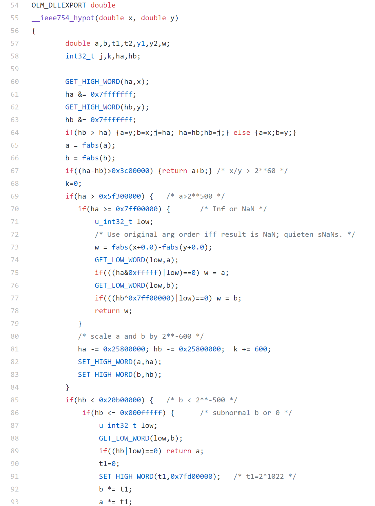
That’s what bullet-proof, bug checked, has been compiled on every platform you can imagine and survived code looks like.
There’s more!
Active Research
When I learned how complex production versions of hypot could be, I shouted out about it on twitter and learned that the story of hypot was far from over!
The implementation of the hypot function is still a matter of active research! See the paper here https://arxiv.org/abs/1904.09481

Is Your Research Software Correct?
Given that such a ‘simple’ computation is so complicated to implement well, consider your own code and ask Is Your Research Software Correct?.
Audiences can be brutal
I still have nightmares about the first talk I ever gave as a PhD student. I was not a strong presenter, my grasp of the subject matter was still very tenuous and I was as nervous as hell. Six months or so into my studentship, I was to give a survey of the field I was studying to a bunch of very experienced researchers. I spent weeks preparing…practicing…honing my slides…hoping that it would all be good enough.
The audience was not kind to me! Even though it was only a small group of around 12 people, they were brutal! I felt like they leaped upon every mistake I made, relished in pointing out every misunderstanding I had and all-round gave me a very hard time. I had nothing like the robustness I have now and very nearly quit my PhD the very next day. I can only thank my office mates and enough beer to kill a pony for collectively talking me out of quitting.
I remember stopping three quarters of the way through saying ‘That’s all I want to say on the subject’ only for one of the senior members of the audience to point out that ‘You have not talked about all the topics you promised’. He made me go back to the slide that said something like ‘Things I will talk about’ or ‘Agenda’ or whatever else I called the stupid thing and say ‘Look….you’ve not mentioned points X,Y and Z’ [1].
Everyone agreed and so my torture continued for another 15 minutes or so.
Practice makes you tougher
Since that horrible day, I have given hundreds of talks to audiences that range in size from 5 up to 300+ and this amount of practice has very much changed how I view these events. I always enjoy them…always! Even when they go badly!
In the worst case scenario, the most that can happen is that I get given a mildly bad time for an hour or so of my life but I know I’ll get over it. I’ve gotten over it before. No big deal! Academic presentations on topics such as research computing rarely lead to life threatening outcomes.
But what if it was recorded?!
Anyone who has worked with me for an appreciable amount of time will know of my pathological fear of having one of my talks recorded. Point a camera at me and the confident, experienced speaker vanishes and is replaced by someone much closer to the terrified PhD student of my youth.
I struggle to put into words what I’m so afraid of but I wonder if it ultimately comes down to the fact that if that PhD talk had been recorded and put online, I would never have been able to get away from it. My humiliation would be there for all to see…forever.
JuliaCon 2018 and Rise of the Research Software Engineer
When the organizers of JuliaCon 2018 invited me to be a keynote speaker on the topic of Research Software Engineering, my answer was an enthusiastic ‘Yes’. As soon as I learned that they would be live streaming and recording all talks, however, my enthusiasm was greatly dampened.
‘Would you mind if my talk wasn’t live streamed and recorded’ I asked them. ‘Sure, no problem’ was the answer….
Problem averted. No need to face my fears this week!
A fellow delegate of the conference pointed out to me that my talk would be the only one that wouldn’t be on the live stream. That would look weird and not in a good way.
‘Can I just be live streamed but not recorded’ I asked the organisers. ‘Sure, no problem’ [2] was the reply….
Later on the technician told me that I could have it recorded but it would be instantly hidden from the world until I had watched it and agreed it wasn’t too terrible. Maybe this would be a nice first step in my record-a-talk-a-phobia therapy he suggested.
So…on I went and it turned out not to be as terrible as I had imagined it might be. So we published it. I learned that I say ‘err’ and ‘um’ a lot [3] which I find a little embarrassing but perhaps now that I know I have that problem, it’s something I can work on.
Rise of the Research Software Engineer
Anyway, here’s the video of the talk. It’s about some of the history of The Research Software Engineering movement and how I worked with some awesome people at The University of Sheffield to create a RSE group. If you are the computer-person in your research group who likes software more than papers, you may be one of us. Come join the tribe!
Slide deck at mikecroucher.github.io/juliacon2018/
Feel free to talk to me on twitter about it: @walkingrandomly
Thanks to the infinitely patient and wonderful organisers of JuliaCon 2018 for the opportunity to beat one of my long standing fears.
Footnotes
[1] Pro-Tip: Never do one of these ‘Agenda’ slides…give yourself leeway to alter the course of your presentation midway through depending on how well it is going.
[2] So patient! Such a lovely team!
[3] Like A LOT! My mum watched the video and said ‘No idea what you were talking about but OMG can you cut out the ummms and ahhs’
A question I get asked a lot is ‘How can I do nonlinear least squares curve fitting in X?’ where X might be MATLAB, Mathematica or a whole host of alternatives. Since this is such a common query, I thought I’d write up how to do it for a very simple problem in several systems that I’m interested in
This is the Julia version. For other versions,see the list below
- Simple nonlinear least squares curve fitting in Maple
- Simple nonlinear least squares curve fitting in Mathematica
- Simple nonlinear least squares curve fitting in MATLAB
- Simple nonlinear least squares curve fitting in Python
- Simple nonlinear least squares curve fitting in R
The problem
xdata = -2,-1.64,-1.33,-0.7,0,0.45,1.2,1.64,2.32,2.9
ydata = 0.699369,0.700462,0.695354,1.03905,1.97389,2.41143,1.91091,0.919576,-0.730975,-1.42001
and you’d like to fit the function

using nonlinear least squares. You’re starting guesses for the parameters are p1=1 and P2=0.2
For now, we are primarily interested in the following results:
- The fit parameters
- Sum of squared residuals
Future updates of these posts will show how to get other results such as confidence intervals. Let me know what you are most interested in.
Julia solution using Optim.jl
Optim.jl is a free Julia package that contains a suite of optimisation routines written in pure Julia. If you haven’t done so already, you’ll need to install the Optim package
Pkg.add("Optim")
The solution is almost identical to the example given in the curve fitting demo of the Optim.jl readme file:
using Optim

model(xdata,p) = p[1]*cos(p[2]*xdata)+p[2]*sin(p[1]*xdata)

xdata = [-2,-1.64,-1.33,-0.7,0,0.45,1.2,1.64,2.32,2.9]
ydata = [0.699369,0.700462,0.695354,1.03905,1.97389,2.41143,1.91091,0.919576,-0.730975,-1.42001]

beta, r, J = curve_fit(model, xdata, ydata, [1.0, 0.2])
# beta = best fit parameters
# r = vector of residuals
# J = estimated Jacobian at solution

@printf("Best fit parameters are: %f and %f",beta[1],beta[2])
@printf("The sum of squares of residuals is %f",sum(r.^2.0))
The result is
Best fit parameters are: 1.881851 and 0.700230
@printf("The sum of squares of residuals is %f",sum(r.^2.0))
Notes
I used Julia version 0.2 on 64bit Windows 7 to run the code in this post
From the wikipedia page on Division by Zero: “The IEEE 754 standard specifies that every floating point arithmetic operation, including division by zero, has a well-defined result”.
MATLAB supports this fully:
>> 1/0
ans =
   Inf
>> 1/(-0)
ans =
  -Inf
>> 0/0
ans =
   NaN
Julia is almost there, but doesn’t handled the signed 0 correctly (This is using Version 0.2.0-prerelease+3768 on Windows)
julia> 1/0
Inf

julia> 1/(-0)
Inf

julia> 0/0
NaN
Python throws an exception. (Python 2.7.5 using IPython shell)
In [4]: 1.0/0.0
---------------------------------------------------------------------------
ZeroDivisionError                         Traceback (most recent call last)
 in ()
----> 1 1.0/0.0

ZeroDivisionError: float division by zero

In [5]: 1.0/(-0.0)
---------------------------------------------------------------------------
ZeroDivisionError                         Traceback (most recent call last)
 in ()
----> 1 1.0/(-0.0)

ZeroDivisionError: float division by zero

In [6]: 0.0/0.0
---------------------------------------------------------------------------
ZeroDivisionError                         Traceback (most recent call last)
 in ()
----> 1 0.0/0.0

ZeroDivisionError: float division by zero
Update:
Julia does do things correctly, provided I make it clear that I am working with floating point numbers:
julia> 1.0/0.0
Inf

julia> 1.0/(-0.0)
-Inf

julia> 0.0/0.0
NaN
I support scientific applications at The University of Manchester (see my LinkedIn profile if you’re interested in the details) and part of my job involves working on code written by researchers in a variety of languages. When I say ‘variety’ I really mean it – MATLAB, Mathematica, Python, C, Fortran, Julia, Maple, Visual Basic and PowerShell are some languages I’ve worked with this month for instance.
Having to juggle the semantics of so many languages in my head sometimes leads to momentary confusion when working on someone’s program. For example, I’ve been doing a lot of Python work recently but this morning I was hacking away on someone’s MATLAB code. Buried deep within the program, it would have been very sensible to be able to do the equivalent of this:
a=rand(3,3)

a =
    0.8147    0.9134    0.2785
    0.9058    0.6324    0.5469
    0.1270    0.0975    0.9575

>> [x,y,z]=a(:,1)

Indexing cannot yield multiple results.
That is, I want to be able to take the first column of the matrix a and broadcast it out to the variables x,y and z. The code I’m working on uses MUCH bigger matrices and this kind of assignment is occasionally useful since the variable names x,y,z have slightly more meaning than a(1,3), a(2,3), a(3,3).
The only concise way I’ve been able to do something like this using native MATLAB commands is to first convert to a cell. In MATLAB 2013a for instance:
>> temp=num2cell(a(:,1));
>> [x y z] = temp{:}

x =
    0.8147

y =
    0.9058

z =
    0.1270
This works but I think it looks ugly and introduces conversion overheads. The problem I had for a short time is that I subconsciously expected multiple assignment to ‘Just Work’ in MATLAB since the concept makes sense in several other languages I use regularly.
from pylab import rand
a=rand(3,3)
[a,b,c]=a[:,0]
a = RandomReal[1, {3, 3}]
{x,y,z}=a[[All,1]]
a=rand(3,3);
(x,y,z)=a[:,1]
I’ll admit that I don’t often need this construct in MATLAB but it would definitely be occasionally useful. I wonder what other opinions there are out there? Do you think multiple assignment is useful (in any language)?
I felt like playing with Julia and MATLAB this Sunday morning. I found some code that prices European Options in MATLAB using Monte Carlo simulations over at computeraidedfinance.com and thought that I’d port this over to Julia. Here’s the original MATLAB code
function V = bench_CPU_European(numPaths)
%Simple European
steps = 250;
r = (0.05);
sigma = (0.4);
T = (1);
dt = T/(steps);
K = (100);

S = 100 * ones(numPaths,1);

for i=1:steps
 rnd = randn(numPaths,1);
 S = S .* exp((r-0.5*sigma.^2)*dt + sigma*sqrt(dt)*rnd);
end
V = mean( exp(-r*T)*max(K-S,0) )
I ran this a couple of times to see what results I should be getting and how long it would take for 1 million paths:
tic;bench_CPU_European(1000000);toc
V =
   13.1596
Elapsed time is 6.035635 seconds.
>> tic;bench_CPU_European(1000000);toc
V =
   13.1258
Elapsed time is 5.924104 seconds.
>> tic;bench_CPU_European(1000000);toc
V =
   13.1479
Elapsed time is 5.936475 seconds.
The result varies because this is a stochastic process but we can see that it should be around 13.1 or so and takes around 6 seconds on my laptop. Since it’s Sunday morning, I am feeling lazy and have no intention of considering if this code is optimal or not right now. I’m just going to copy and paste it into a julia file and hack at the syntax until it becomes valid Julia code. The following seems to work
function bench_CPU_European(numPaths)

steps = 250
r = 0.05
sigma = .4;
T = 1;
dt = T/(steps)
K = 100;

S = 100 * ones(numPaths,1);

for i=1:steps
 rnd = randn(numPaths,1)
 S = S .* exp((r-0.5*sigma.^2)*dt + sigma*sqrt(dt)*rnd)
end
V = mean( exp(-r*T)*max(K-S,0) )
end
I ran this on Julia and got the following
julia> tic();bench_CPU_European(1000000);toc()
elapsed time: 36.259000062942505 seconds
36.259000062942505

julia> bench_CPU_European(1000000)
13.114855104505445
The Julia code appears to be valid, it gives the correct result of 13.1 ish but at 36.25 seconds is around 6 times slower than the MATLAB version. The dog needs walking so I’m going to think about this another time but comments are welcome.
Update (9pm 7th October 2012): I’ve just tried this Julia code on the Linux partition of the same laptop and 1 million paths took 14 seconds or so:
tic();bench_CPU_European(1000000);toc()
elapsed time: 14.146281957626343 seconds
I built this version of Julia from source and so it’s at the current bleeding edge (version 0.0.0+98589672.r65a1 Commit 65a1f3dedc (2012-10-07 06:40:18). The code is still slower than the MATLAB version but better than the older Windows build
Update: 13th October 2012
Over on the Julia mailing list, someone posted a faster version of this simulation in Julia
function bench_eu(numPaths)
    steps = 250
    r = 0.05
    sigma = .4;
    T = 1;
    dt = T/(steps)
    K = 100;

    S = 100 * ones(numPaths,1);

    t1 = (r-0.5*sigma.^2)*dt
    t2 = sigma*sqrt(dt)
    for i=1:steps
        for j=1:numPaths
            S[j] .*= exp(t1 + t2*randn())
        end
    end

    V = mean( exp(-r*T)*max(K-S,0) )
end
On the Linux partition of my test machine, this got through 1000000 paths in 8.53 seconds, very close to the MATLAB speed:
julia> tic();bench_eu(1000000);toc()
elapsed time: 8.534484148025513 seconds
It seems that, when using Julia, one needs to unlearn everything you’ve ever learned about vectorisation in MATLAB.
Update: 28th October 2012
Members of the Julia team have been improving the performance of the randn() function used in the above code (see here and here for details). Using the de-vectorised code above, execution time for 1 million paths in Julia is now down to 7.2 seconds on my machine on Linux. Still slower than the MATLAB 2012a implementation but it’s getting there. This was using Julia version 0.0.0+100403134.r0999 Commit 099936aec6 (2012-10-28 05:24:40)
tic();bench_eu(1000000);toc()
elapsed time: 7.223690032958984 seconds
7.223690032958984
- Laptop model: Dell XPS L702X
- CPU:Intel Core i7-2630QM @2Ghz software overclockable to 2.9Ghz. 4 physical cores but total 8 virtual cores due to Hyperthreading.
- RAM: 8 Gb
- OS: Windows 7 Home Premium 64 bit and Ubuntu 12.04
- MATLAB: 2012a
- Julia: Original windows version was Version 0.0.0+94063912.r17f5, Commit 17f50ea4e0 (2012-08-15 22:30:58). Several versions used on Linux since, see text for details.
I first mentioned Julia, a new language for high performance scientific computing, back in the February edition of a Month of Math software and it certainly hasn’t stood still since then. A WalkingRandomly reader, Ohad, recently contacted me to tell me about a forum post announcing some Julia speed improvements.
Julia has a set of micro-benchmarks and the slowest of them is now only two times slower than the equivalent in C. That’s compiled language performance with an easy to use scripting language. Astonishingly, Julia is faster than gfortran in a couple of instances. Nice work!
Comparison times between Julia and other scientific scripting languages (MATLAB, Python and R for instance) for these micro-benchmarks are posted on Julia’s website. The Julia team have included the full benchmark source code used for all languages so if you are an expert in one of them, why not take a look at how they have represented your language and see what you think?
Let me know if you’ve used Julia at all, I’m interested in what people think of it.