
Archive for the ‘Linear Algebra’ Category
I recently wrote a blog post for my new employer, The Numerical Algorithms Group, called Exploiting Matrix Structure in the solution of linear systems. It’s a demonstration that shows how choosing the right specialist solver for your problem rather than using a general purpose one can lead to a speed up of well over 100 times! The example is written in Python but the NAG routines used can be called from a range of languages including C,C++, Fortran, MATLAB etc etc
I’m working on optimising some R code written by a researcher at University of Sheffield and its very much a war of attrition! There’s no easily optimisable hotspot and there’s no obvious way to leverage parallelism. Progress is being made by steadily identifying places here and there where we can do a little better. 10% here and 20% there can eventually add up to something worth shouting about.
One such micro-optimisation we discovered involved multiplying two matrices together where one of them needed to be transposed. Here’s a minimal example.
#Set random seed for reproducibility
set.seed(3)

# Generate two random n by n matrices
n = 10
a = matrix(runif(n*n,0,1),n,n)
b = matrix(runif(n*n,0,1),n,n)

# Multiply the matrix a by the transpose of b
c = a %*% t(b)
When the speed of linear algebra computations are an issue in R, it makes sense to use a version that is linked to a fast implementation of BLAS and LAPACK and we are already doing that on our HPC system.
Here, I am using version 3.3.3 of Microsoft R Open which links to Intel’s MKL (an implementation of BLAS and LAPACK) on a Windows laptop.
In R, there is another way to do the computation c = a %*% t(b) — we can make use of the tcrossprod function (There is also a crossprod function for when you want to do t(a) %*% b)
c_new = tcrossprod(a,b)
Let’s check for equality
c_new == c
[,1] [,2] [,3] [,4] [,5] [,6] [,7] [,8] [,9] [,10]
[1,] TRUE TRUE TRUE TRUE TRUE TRUE TRUE TRUE TRUE TRUE
[2,] TRUE TRUE TRUE TRUE TRUE TRUE TRUE TRUE TRUE TRUE
[3,] TRUE TRUE TRUE TRUE TRUE TRUE TRUE TRUE TRUE TRUE
[4,] TRUE TRUE TRUE TRUE TRUE TRUE TRUE TRUE TRUE TRUE
[5,] TRUE TRUE TRUE TRUE TRUE TRUE TRUE TRUE TRUE TRUE
[6,] TRUE TRUE TRUE TRUE TRUE TRUE TRUE TRUE TRUE TRUE
[7,] TRUE TRUE TRUE TRUE TRUE TRUE TRUE TRUE TRUE TRUE
[8,] TRUE TRUE TRUE TRUE TRUE TRUE TRUE TRUE TRUE TRUE
[9,] TRUE TRUE TRUE TRUE TRUE TRUE TRUE TRUE TRUE TRUE
[10,] TRUE TRUE TRUE TRUE TRUE TRUE TRUE TRUE TRUE TRUE
Sometimes, when comparing the two methods you may find that some of those entries are FALSE which may worry you!
If that happens, computing the difference between the two results should convince you that all is OK and that the differences are just because of numerical noise. This happens sometimes when dealing with floating point arithmetic (For example, see https://www.walkingrandomly.com/?p=5380).
Let’s time the two methods using the microbenchmark package.
install.packages('microbenchmark')
library(microbenchmark)
We time just the matrix multiplication part of the code above:
microbenchmark(
original = a %*% t(b),
tcrossprod = tcrossprod(a,b)
)


Unit: nanoseconds
expr min lq mean median uq max neval
original 2918 3283 3491.312 3283 3647 18599 1000
tcrossprod 365 730 756.278 730 730 10576 1000
We are only saving microseconds here but that’s more than a factor of 4 speed-up in this small matrix case. If that computation is being performed a lot in a tight loop (and for our real application, it was), it can add up to quite a difference.
As the matrices get bigger, the speed-benefit in percentage terms gets lower but tcrossprod always seems to be the faster method. For example, here are the results for 1000 x 1000 matrices
#Set random seed for reproducibility
set.seed(3)

# Generate two random n by n matrices
n = 1000
a = matrix(runif(n*n,0,1),n,n)
b = matrix(runif(n*n,0,1),n,n)

microbenchmark(
original = a %*% t(b),
tcrossprod = tcrossprod(a,b)
)

Unit: milliseconds
expr min lq mean median uq max neval
original 18.93015 26.65027 31.55521 29.17599 31.90593 71.95318 100
tcrossprod 13.27372 18.76386 24.12531 21.68015 23.71739 61.65373 100
The cost of not using an optimised version of BLAS and LAPACK
While writing this blog post, I accidentally used the CRAN version of R. The recently released version 3.4. Unlike Microsoft R Open, this is not linked to the Intel MKL and so matrix multiplication is rather slower.
For our original 10 x 10 matrix example we have:
library(microbenchmark)
#Set random seed for reproducibility
set.seed(3)

# Generate two random n by n matrices
n = 10
a = matrix(runif(n*n,0,1),n,n)
b = matrix(runif(n*n,0,1),n,n)

microbenchmark(
original = a %*% t(b),
tcrossprod = tcrossprod(a,b)
)

Unit: microseconds
       expr   min    lq    mean median     uq    max neval
   original 3.647 3.648 4.22727  4.012 4.1945 22.611   100
 tcrossprod 1.094 1.459 1.52494  1.459 1.4600  3.282   100
Everything is a little slower as you might expect and the conclusion of this article — tcrossprod(a,b) is faster than a %*% t(b) — seems to still be valid.
However, when we move to 1000 x 1000 matrices, this changes
library(microbenchmark)
#Set random seed for reproducibility
set.seed(3)

# Generate two random n by n matrices
n = 1000
a = matrix(runif(n*n,0,1),n,n)
b = matrix(runif(n*n,0,1),n,n)

microbenchmark(
original = a %*% t(b),
tcrossprod = tcrossprod(a,b)
)

Unit: milliseconds
       expr      min       lq     mean   median       uq       max neval
   original 546.6008 587.1680 634.7154 602.6745 658.2387  957.5995   100
 tcrossprod 560.4784 614.9787 658.3069 634.7664 685.8005 1013.2289   100
As expected, both results are much slower than when using the Intel MKL-lined version of R (~600 milliseconds vs ~31 milliseconds) — nothing new there. More disappointingly, however, is that now tcrossprod is slightly slower than explicitly taking the transpose.
As such, this particular micro-optimisation might not be as effective as we might like for all versions of R.
For a while now, Microsoft have provided a free Jupyter Notebook service on Microsoft Azure. At the moment they provide compute kernels for Python, R and F# providing up to 4Gb of memory per session. Anyone with a Microsoft account can upload their own notebooks, share notebooks with others and start computing or doing data science for free.
They University of Cambridge uses them for teaching, and they’ve also been used by the LIGO people (gravitational waves) for dissemination purposes.
This got me wondering. How much power does Microsoft provide for free within these notebooks? Computing is pretty cheap these days what with the Raspberry Pi and so on but what do you get for nothing? The memory limit is 4GB but how about the computational power?
To find out, I created a simple benchmark notebook that finds out how quickly a computer multiplies matrices together of various sizes.
- The benchmark notebook is here on Azure https://notebooks.azure.com/walkingrandomly/libraries/MatrixMatrix
- and here on GitHub https://github.com/mikecroucher/Jupyter-Matrix-Matrix
Matrix-Matrix multiplication is often used as a benchmark because it’s a common operation in many scientific domains and it has been optimised to within an inch of it’s life. I have lost count of the number of times where my contribution to a researcher’s computational workflow has amounted to little more than ‘don’t multiply matrices together like that, do it like this…it’s much faster’
So how do Azure notebooks perform when doing this important operation? It turns out that they max out at 263 Gigaflops! 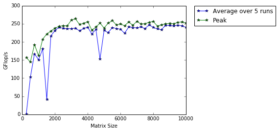
For context, here are some other results:
- A 16 core Intel Xeon E5-2630 v3 node running on Sheffield’s HPC system achieved around 500 Gigaflops.
- My mid-2014 Mabook Pro, with a Haswell Intel CPU hit, hit 169 Gigaflops.
- My Dell XPS9560 laptop, with a Kaby Lake Intel CPU, manages 153 Gigaflops.
As you can see, we are getting quite a lot of compute power for nothing from Azure Notebooks. Of course, one of the limiting factors of the free notebook service is that we are limited to 4GB of RAM but that was more than I had on my own laptops until 2011 and I got along just fine.
Another fun fact is that according to https://www.top500.org/statistics/perfdevel/, 263 Gigaflops would have made it the fastest computer in the world until 1994. It would have stayed in the top 500 supercomputers of the world until June 2003 [1].
Not bad for free!
[1] The top 500 list is compiled using a different benchmark called LINPACK so a direct comparison isn’t strictly valid…I’m using a little poetic license here.
Linear Algebra – Foundations to Frontiers (or LAFF to its friends) is a popular, high quality and free MOOC that, as the title suggests, teaches aspects of linear algebra in a way that takes the student from the very basics through to some cutting edge techniques. I worked through much of it last year and thoroughly enjoyed the approach it took — focusing on programming aspects from the very beginning. The course authors are also among the developers of the FLAME project, a high performance linear algebra library, and one of the interesting aspects of the LAFF course (for me at least) was that it taught linear algebra in a way that also allowed you to understand the approaches used in the algorithms behind FLAME.
Last year, all of the programming assignments in LAFF were done in Python, making use of the IPython notebook. This year, the software stack will be different and will be based on MATLAB. I understand that everyone who signs up to LAFF will be able to get a free MATLAB license from Mathworks for the duration of the course. Understandably, this caused quite a bit of discussion between the LAFF team and software/language geeks like me. In a recent Facebook thread, I asked about the switch and received the reply
‘MATLAB will be free during the course. There are open source equivalents, but Mathworks staff is supporting the use of MATLAB (staff for us). There were some who never got the IPython notebooks to work properly. We are really excited at the opportunity to innovate again and perhaps clear up snags in the programming issues we had. It was complicated to support IPython on all of the operating systems and machines that participants use. MATLAB promises to be easier and will allow us again to concentrate on the Linear Algebra’ – LAFF UTx
I’m sufficiently interested in this change from IPython to MATLAB that I’ll be signing up for the course again this year and I encourage you to do the same — I believe that the programming-centric teaching approach taken by LAFF is extremely well done and your time would be well-spent working through the course.
The course starts on 28th January 2015 so sign up now!
Here’s the trailer for last year’s course.
Given a symmetric matrix such as
![\light \[ \left( \begin{array}{ccc} 1 & 1 & 0 \\ 1 & 1 & 1 \\ 0 & 1 & 1 \end{array} \right)\]](http://walkingrandomly.com/wp-content/ql-cache/quicklatex.com-0ba648b6b45c6e624aefe7341a911896_l3.png "Rendered by QuickLaTeX.com")
What’s the nearest correlation matrix? A 2002 paper by Manchester University’s Nick Higham which answered this question has turned out to be rather popular! At the time of writing, Google tells me that it’s been cited 394 times.
Last year, Nick wrote a blog post about the algorithm he used and included some MATLAB code. He also included links to applications of this algorithm and implementations of various NCM algorithms in languages such as MATLAB, R and SAS as well as details of the superb commercial implementation by The Numerical algorithms group.
I noticed that there was no Python implementation of Nick’s code so I ported it myself.
Here’s an example IPython session using the module
In [1]: from nearest_correlation import nearcorr

In [2]: import numpy as np

In [3]: A = np.array([[2, -1, 0, 0],
   ...:               [-1, 2, -1, 0],
   ...:               [0, -1, 2, -1],
   ...:               [0, 0, -1, 2]])

In [4]: X = nearcorr(A)

In [5]: X
Out[5]:
array([[ 1.        , -0.8084125 ,  0.1915875 ,  0.10677505],
       [-0.8084125 ,  1.        , -0.65623269,  0.1915875 ],
       [ 0.1915875 , -0.65623269,  1.        , -0.8084125 ],
       [ 0.10677505,  0.1915875 , -0.8084125 ,  1.        ]])
This module is in the early stages and there is a lot of work to be done. For example, I’d like to include a lot more examples in the test suite, add support for the commercial routines from NAG and implement other algorithms such as the one by Qi and Sun among other things.
Hopefully, however, it is just good enough to be useful to someone. Help yourself and let me know if there are any problems. Thanks to Vedran Sego for many useful comments and suggestions.
- github repository for the Python NCM module, nearest_correlation
- Nick Higham’s original MATLAB code.
- NAG’s commercial implementation – callable from C, Fortran, MATLAB, Python and more. A superb implementation that is significantly faster and more robust than this one!
In a recent Stack Overflow query, someone asked if you could switch off the balancing step when calculating eigenvalues in Python. In the document A case where balancing is harmful, David S. Watkins describes the balancing step as ‘the input matrix A is replaced by a rescaled matrix A* = D-1AD, where D is a diagonal matrix chosen so that, for each i, the ith row and the ith column of A* have roughly the same norm.’
Such balancing is usually very useful and so is performed by default by software such as MATLAB or Numpy. There are times, however, when one would like to switch it off.
In MATLAB, this is easy and the following is taken from the online MATLAB documentation
A = [ 3.0     -2.0      -0.9     2*eps;
     -2.0      4.0       1.0    -eps;
     -eps/4    eps/2    -1.0     0;
     -0.5     -0.5       0.1     1.0];

[VN,DN] = eig(A,'nobalance')
VN =

    0.6153   -0.4176   -0.0000   -0.1528
   -0.7881   -0.3261         0    0.1345
   -0.0000   -0.0000   -0.0000   -0.9781
    0.0189    0.8481   -1.0000    0.0443

DN =
    5.5616         0         0         0
         0    1.4384         0         0
         0         0    1.0000         0
         0         0         0   -1.0000
At the time of writing, it is not possible to directly do this in Numpy (as far as I know at least). Numpy’s eig command currently uses the LAPACK routine DGEEV to do the heavy lifting for double precision matrices. We can see this by looking at the source code of numpy.linalg.eig where the relevant subsection is
lapack_routine = lapack_lite.dgeev
        wr = zeros((n,), t)
        wi = zeros((n,), t)
        vr = zeros((n, n), t)
        lwork = 1
        work = zeros((lwork,), t)
        results = lapack_routine(_N, _V, n, a, n, wr, wi,
                                  dummy, 1, vr, n, work, -1, 0)
        lwork = int(work[0])
        work = zeros((lwork,), t)
        results = lapack_routine(_N, _V, n, a, n, wr, wi,
                                  dummy, 1, vr, n, work, lwork, 0)
My plan was to figure out how to tell DGEEV not to perform the balancing step and I’d be done. Sadly, however, it turns out that this is not possible. Taking a look at the reference implementation of DGEEV, we can see that the balancing step is always performed and is not user controllable–here’s the relevant bit of Fortran
*     Balance the matrix
*     (Workspace: need N)
*
      IBAL = 1
      CALL DGEBAL( 'B', N, A, LDA, ILO, IHI, WORK( IBAL ), IERR )
So, using DGEEV is a dead-end unless we are willing to modifiy and recompile the lapack source — something that’s rarely a good idea in my experience. There is another LAPACK routine that is of use, however, in the form of DGEEVX that allows us to control balancing. Unfortunately, this routine is not part of the numpy.linalg.lapack_lite interface provided by Numpy and I’ve yet to figure out how to add extra routines to it.
I’ve also discovered that this functionality is an open feature request in Numpy.
Enter the NAG Library
My University has a site license for the commercial Numerical Algorithms Group (NAG) library. Among other things, NAG offers an interface to all of LAPACK along with an interface to Python. So, I go through the installation and do
import numpy as np
from ctypes import *
from nag4py.util import Nag_RowMajor,Nag_NoBalancing,Nag_NotLeftVecs,Nag_RightVecs,Nag_RCondEigVecs,Integer,NagError,INIT_FAIL
from nag4py.f08 import nag_dgeevx

eps = np.spacing(1)
np.set_printoptions(precision=4,suppress=True)

def unbalanced_eig(A):
    """
    Compute the eigenvalues and right eigenvectors of a square array using DGEEVX via the NAG library.
    Requires the NAG C library and NAG's Python wrappers http://www.nag.co.uk/python.asp
    The balancing step that's performed in DGEEV is not performed here.
    As such, this function is the same as the MATLAB command eig(A,'nobalance')

    Parameters
    ----------
    A : (M, M) Numpy array
        A square array of real elements.

        On exit:
        A is overwritten and contains the real Schur form of the balanced version of the input matrix .

    Returns
    -------
    w : (M,) ndarray
        The eigenvalues
    v : (M, M) ndarray
        The eigenvectors

    Author: Mike Croucher (www.walkingrandomly.com)
    Testing has been mimimal
    """

    order = Nag_RowMajor
    balanc = Nag_NoBalancing
    jobvl = Nag_NotLeftVecs
    jobvr = Nag_RightVecs
    sense = Nag_RCondEigVecs

    n = A.shape[0]
    pda = n
    pdvl = 1

    wr = np.zeros(n)
    wi = np.zeros(n)

    vl=np.zeros(1);
    pdvr = n
    vr = np.zeros(pdvr*n)

    ilo=c_long(0)
    ihi=c_long(0)

    scale = np.zeros(n)
    abnrm = c_double(0)
    rconde = np.zeros(n)
    rcondv = np.zeros(n)

    fail = NagError()
    INIT_FAIL(fail)

    nag_dgeevx(order,balanc,jobvl,jobvr,sense,
               n, A.ctypes.data_as(POINTER(c_double)), pda, wr.ctypes.data_as(POINTER(c_double)),
               wi.ctypes.data_as(POINTER(c_double)),vl.ctypes.data_as(POINTER(c_double)),pdvl,
               vr.ctypes.data_as(POINTER(c_double)),pdvr,ilo,ihi, scale.ctypes.data_as(POINTER(c_double)),
               abnrm, rconde.ctypes.data_as(POINTER(c_double)),rcondv.ctypes.data_as(POINTER(c_double)),fail)

    if all(wi == 0.0):
            w = wr
            v = vr.reshape(n,n)
    else:
            w = wr+1j*wi
            v = array(vr, w.dtype).reshape(n,n)

    return(w,v)
Define a test matrix:
A = np.array([[3.0,-2.0,-0.9,2*eps],
          [-2.0,4.0,1.0,-eps],
          [-eps/4,eps/2,-1.0,0],
          [-0.5,-0.5,0.1,1.0]])
Do the calculation
(w,v) = unbalanced_eig(A)
which gives
(array([ 5.5616,  1.4384,  1.    , -1.    ]),
 array([[ 0.6153, -0.4176, -0.    , -0.1528],
       [-0.7881, -0.3261,  0.    ,  0.1345],
       [-0.    , -0.    , -0.    , -0.9781],
       [ 0.0189,  0.8481, -1.    ,  0.0443]]))
This is exactly what you get by running the MATLAB command eig(A,’nobalance’).
Note that unbalanced_eig(A) changes the input matrix A to
array([[ 5.5616, -0.0662,  0.0571,  1.3399],
       [ 0.    ,  1.4384,  0.7017, -0.1561],
       [ 0.    ,  0.    ,  1.    , -0.0132],
       [ 0.    ,  0.    ,  0.    , -1.    ]])
According to the NAG documentation, this is the real Schur form of the balanced version of the input matrix. I can’t see how to ask NAG to not do this. I guess that if it’s not what you want unbalanced_eig() to do, you’ll need to pass a copy of the input matrix to NAG.
The IPython notebook
The code for this article is available as an IPython Notebook
The future
This blog post was written using Numpy version 1.7.1. There is an enhancement request for the functionality discussed in this article open in Numpy’s git repo and so I expect this article to become redundant pretty soon.
Last week I gave a live demo of the IPython notebook to a group of numerical analysts and one of the computations we attempted to do was to solve the following linear system using Numpy’s solve command.

Now, the matrix shown above is singular and so we expect that we might have problems. Before looking at how Numpy deals with this computation, lets take a look at what happens if you ask MATLAB to do it
>> A=[1 2 3;4 5 6;7 8 9];
>> b=[15;15;15];
>> x=A\b
Warning: Matrix is close to singular
or badly scaled. Results may be
inaccurate. RCOND =  1.541976e-18.
x =
  -39.0000
   63.0000
  -24.0000
MATLAB gives us a warning that the input matrix is close to being singular (note that it didn’t actually recognize that it is singular) along with an estimate of the reciprocal of the condition number. It tells us that the results may be inaccurate and we’d do well to check. So, lets check:
>> A*x

ans =
   15.0000
   15.0000
   15.0000

>> norm(A*x-b)

ans =
2.8422e-14
We seem to have dodged the bullet since, despite the singular nature of our matrix, MATLAB has able to find a valid solution. MATLAB was right to have warned us though…in other cases we might not have been so lucky.
Let’s see how Numpy deals with this using the IPython notebook:
In [1]:
import numpy
from numpy import array
from numpy.linalg import solve
A=array([[1,2,3],[4,5,6],[7,8,9]])
b=array([15,15,15])
solve(A,b)

Out[1]:

array([-39.,  63., -24.])
It gave the same result as MATLAB [See note 1], presumably because it’s using the exact same LAPACK routine, but there was no warning of the singular nature of the matrix. During my demo, it was generally felt by everyone in the room that a warning should have been given, particularly when working in an interactive setting.
If you look at the documentation for Numpy’s solve command you’ll see that it is supposed to throw an exception when the matrix is singular but it clearly didn’t do so here. The exception is sometimes thrown though:
In [4]:

C=array([[1,1,1],[1,1,1],[1,1,1]])
x=solve(C,b)

---------------------------------------------------------------------------
LinAlgError                               Traceback (most recent call last)
 in ()
      1 C=array([[1,1,1],[1,1,1],[1,1,1]])
----> 2 x=solve(C,b)

C:\Python32\lib\site-packages\numpy\linalg\linalg.py in solve(a, b)
    326     results = lapack_routine(n_eq, n_rhs, a, n_eq, pivots, b, n_eq, 0)
    327     if results['info'] > 0:
--> 328         raise LinAlgError('Singular matrix')
    329     if one_eq:
    330         return wrap(b.ravel().astype(result_t))

LinAlgError: Singular matrix
It seems that Numpy is somehow checking for exact singularity but this will rarely be detected due to rounding errors. Those I’ve spoken to consider that MATLAB’s approach of estimating the condition number and warning when that is high would be better behavior since it alerts the user to the fact that the matrix is badly conditioned.
Thanks to Nick Higham and David Silvester for useful discussions regarding this post.
Notes
[1] – The results really are identical which you can see by rerunning the calculation after evaluating format long in MATLAB and numpy.set_printoptions(precision=15) in Python