Walking Randomly

A colleague recently sent me this issue. Consider the following integral

Attempting to evaluate this with Mathematica 9 gives 0:

 f[a_, b_] := Exp[I*(a*x^3 + b*x^2)];
Integrate[f[a, b], {x, -Infinity, Infinity}, 
 Assumptions -> {a > 0, b \[Element] Reals}]

Out[2]= 0

So, for all valid values of a and b, Mathematica tells us that the resulting integral will be 0.

However, Let’s set a=1/3 and b=0 in the function f and ask Mathematica to evaluate that integral

In[3]:= Integrate[f[1/3, 0], {x, -Infinity, Infinity}]

Out[3]= (2*Pi)/(3^(2/3)*Gamma[2/3])

This is definitely not zero as we can see by numerically evaluating the result:

In[5]:=
(2*Pi)/(3^(2/3)*Gamma[2/3])//N

Out[5]= 2.23071

Similarly if we put a=1/3 and b=1 we get another non-zero result

In[7]:= Integrate[f[1/3, 1], {x, -Infinity, Infinity}] // InputForm

Out[7]=2*E^((2*I)/3)*Pi*AiryAi[-1]

In[8]:=
2*E^((2*I)/3)*Pi*AiryAi[-1]//N

Out[8]= 2.64453 + 2.08083 I

We are faced with a situation where Mathematica is disagreeing with itself.  On one hand, it says that the integral is 0 for all a and b but on the other it gives non-zero results for certain combinations of a and b.  Which result do we trust?

One way to proceed would be to use the NIntegrate[] function for the two cases where a and b are explicitly defined.  NIntegrate[] uses completely different algorithms from Integrate.  In particular it uses numerical rather than symbolic methods (apart from some symbolic pre-processing).

NIntegrate[f[1/3, 0], {x, -Infinity, Infinity}]

gives 2.23071 + 0. I and

NIntegrate[f[1/3, 1], {x, -Infinity, Infinity}]

gives 2.64453 + 2.08083 I

What we’ve shown here is that evaluating these integrals using numerical methods gives the same result as evaluating using symbolic methods and numericalizing the result.  This gives me some confidence that its the general, symbolic evaluation that’s incorrect and hence I can file a bug report with Wolfram Research.

Maple 17.01 on the general problem

Since my University has just got a site license for Maple, I wondered what Maple 17.01 would make of the general integral. Using Maple’s 1D input/output we get:

> myint := int(exp(I*(a*x^3+b*x^2)), x = -infinity .. infinity);

myint := (1/12)*3^(1/2)*2^(1/3)*((4/3)*Pi^(5/2)*(((4/27)*I)*b^3/a^2)^(1/3)*exp(((2/27)*I)*b^3/a^2)
*BesselI(-1/3, ((2/27)*I)*b^3/a^2)+((2/3)*I)*Pi^(3/2)*3^(1/2)*b*2^(2/3)
*hypergeom([1/2, 1], [2/3, 4/3],((4/27)*I)*b^3/a^2)/(-I*a)^(2/3)-(8/27)*2^(1/3)*Pi^(5/2)*b^2*
exp(((2/27)*I)*b^3/a^2)*BesselI(1/3, ((2/27)*I)*b^3/a^2)/((-I*a)^(4/3)*(((4/27)*I)*b^3/a^2)^(1/3)))
/(Pi^(3/2)*(-I*a)^(1/3))+(1/12)*3^(1/2)*2^(1/3)*((4/3)*Pi^(5/2)*(((4/27)*I)*b^3/a^2)
^(1/3)*exp(((2/27)*I)*b^3/a^2)*BesselI(-1/3, ((2/27)*I)*b^3/a^2)+((2/3)*I)*Pi^(3/2)*3^(1/2)*b*2^(2/3)
*hypergeom([1/2, 1], [2/3, 4/3], ((4/27)*I)*b^3/a^2)/(I*a)^(2/3)-(8/27)*2^(1/3)*Pi^(5/2)*b^2*
exp(((2/27)*I)*b^3/a^2)*BesselI(1/3, ((2/27)*I)*b^3/a^2)/((I*a)^(4/3)*(((4/27)*I)*b^3/a^2)^(1/3)))
/(Pi^(3/2)*(I*a)^(1/3))

That looks scary! To try to determine if it’s possibly a correct general result, let’s turn this expression into a function and evaluate it for values of a and b we already know the answer to.

>f := unapply(%, a, b):
>result1:=simplify(f(1/3,1));

result1 := (2/27)*3^(1/2)*Pi*exp((2/3)*I)*((-(1/3)*I)^(1/3)*3^(2/3)*(-1)^(1/6)*BesselI(-1/3, (2/3)*I)
+3*(-(1/3)*I)^(2/3)*BesselI(-1/3, (2/3)*I)+3*(-(1/3)*I)^(2/3)*BesselI(1/3, (2/3)*I)-BesselI(1/3, (2/3)*I)
*3^(1/3)*(-1)^(1/3))/(-(1/3)*I)^(2/3)

evalf(result1);
2.644532853+2.080831872*I

Recall that Mathematica returned 2*E^((2*I)/3)*Pi*AiryAi[-1]=2.64453 + 2.08083 I for this case. The numerical results agree to the default precision reported by both packages so I am reasonably confident that Maple’s general solution is correct.

Not so simple simplification?

I am also confident that Maple’s expression involving Bessel functions is equivalent to Mathematica’s expression involving the AiryAi function. I haven’t figured out, however, how to get Maple to automatically reduce the Bessel functions down to AiryAi. I can attempt to go the other way though. In Maple:

>convert(2*exp((2*I)/3)*Pi*AiryAi(-1),Bessel);

(2/3)*exp((2/3)*I)*Pi*(-1)^(1/6)*(-BesselI(1/3, (2/3)*I)*(-1)^(2/3)+BesselI(-1/3, (2/3)*I))

This is more compact than the Bessel function result I get from Maple’s simplify so I guess that Maple’s simplify function could have done a little better here.

Not so general general solution?

Maple’s solution of the general problem should be good for all a and b right?  Let’s try it with a=1/3, b=0

f(1/3,0);
Error, (in BesselI) numeric exception: division by zero

Uh-Oh! So it’s not valid for b=0 then! We know from Mathematica, however, that the solution for this particular case is (2*Pi)/(3^(2/3)*Gamma[2/3])=2.23071. Indeed, if we solve this integral directly in Maple, it agrees with Mathematica

>myint := int(exp(I*(1/3*x^3+0*x^2)), x = -infinity .. infinity);

myint := (2/9)*3^(5/6)*(-1)^(1/6)*Pi/GAMMA(2/3)-(2/9)*3^(5/6)*(-1)^(5/6)*Pi/GAMMA(2/3)

>simplify(myint);
(2/3)*3^(1/3)*Pi/GAMMA(2/3)

>evalf(myint);
2.230707052+0.*I

Going to back to the general result that Maple returned. Although we can’t calculate it directly, We can use limits to see what its value would be at a=1/3, b=0

>simplify(limit(f(1/3, x), x = 0));

(2/9)*Pi*3^(2/3)/((-(1/3)*I)^(1/3)*GAMMA(2/3)*((1/3)*I)^(1/3))

>evalf(%)

evalf(%);
2.230707053+0.1348486379e-9*I

The symbolic expression looks different and we’ve picked up an imaginary part that’s possibly numerical noise. Let’s use more numerical precision to see if we can make the imaginary part go away. 100 digits should do it

>evalf[100](%%);

2.230707051824495741427486519543450239771293806030489125938415383976032081571780278667202004477941904
-0.855678513686459467847075286617333072231119978694352241387724335424279116026690601018858453303153701e-100*I

Well, more precision has made the imaginary part smaller but it’s still there. No matter how much precision I use, it’s always there…getting smaller and smaller as I ramp up the level of precision.

What’s going on?

All I’m doing here is playing around with the same problem in two packages.  Does anyone have any further insights into some of the issues raised?

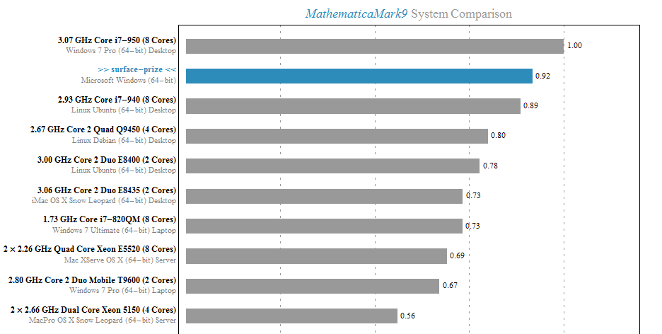
A friend of mine recently got hold of a Microsoft Surface Pro tablet and he let me have a play on it for a couple of hours.  So, I installed Mathematica 9 and ran the benchmark.  A screenshot of the result is below with the Surface’s result in blue.  Not bad for a tablet!

Touch controlled Manipulates were a lot of fun too.  If only I could run such things on my iPad as appeared to be promised in http://blog.wolfram.com/2012/02/17/a-preview-of-cdf-on-ipad/

My only other comment is that the Touch Cover is truly awful, reminding me of ye-olde ZX81, but I’ve been told that the Type Cover is much better

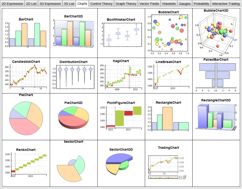
I’m working on a presentation involving Mathematica 9 at the moment and found myself wanting a gallery of all built-in plots using default settings.  Since I couldn’t find such a gallery, I made one myself.  The notebook is available here and includes 99 built-in plots, charts and gauges generated using default settings.  If you hover your mouse over one the plots in the Mathematica notebook, it will display a ToolTip showing usage notes for the function that generated it.

The gallery only includes functions that are fully integrated with Mathematica so doesn’t include things from add-on packages such as StatisticalPlots.

A screenshot of the gallery is below.  I haven’t made an in-browser interactive version due to size.

I was at a seminar yesterday where we were playing with Mathematica and wanted to solve the following equation

1.0609^t == 1.5

You punch this into Mathematica as follows:

Solve[1.0609^t == 1.5]

Mathematica returns the following

During evaluation of In[1]:= Solve::ifun: Inverse functions are being used by Solve, 
so some solutions may not be found; use Reduce for complete solution information. >>

Out[1]= {{t -> 6.85862}}

I have got the solution I expect but Mathematica suggests that I’ll get more information if I use Reduce. So, lets do that.

In[2]:= Reduce[1.0609^t == 1.5, t]
During evaluation of In[2]:= Reduce::ratnz: Reduce was unable to solve the system with inexact 
coefficients. The answer was obtained by solving a corresponding exact system and numericizing the result. >>
Out[20]= C[1] \[Element] Integers && 
  t == -16.9154 (-0.405465 + (0. + 6.28319 I) C[1])

Looks complex and a little complicated! To understand why complex numbers have appeared in the mix you need to know that Mathematica always considers variables to be complex unless you tell it otherwise. So, it has given you the infinite number of complex values of t that would satisfy the original equation. No problem, let’s just tell Mathematica that we are only interested in real values of p.

In[3]:= Reduce[1.0609^t == 1.5, t, Reals]

During evaluation of In[3]:= Reduce::ratnz: Reduce was unable to solve the system with inexact 
coefficients. The answer was obtained by solving a corresponding exact system and numericizing the result. >>

Out[3]= t == 6.85862

Again, I get the solution I expect. However, Mathematica still feels that it is necessary to give me a warning message. Time was ticking on so I posed the question on Mathematica Stack Exchange and we moved on.

http://mathematica.stackexchange.com/questions/19235/why-does-mathematica-struggle-with-solving-this-equation

At the time of writing, the lead answer says that ‘Mathematica is not “struggling” with your equation. The message is simply FYI — to tell you that, for this equation, it prefers to work with exact quantities rather than inexact quantities (reals)’

I’d accept this as an explanation except for one thing; the message say’s that it is UNABLE to solve the equation as I originally posed it and so needs to proceed by solving a corresponding exact system. That implies that it has struggled a great deal, given up and tried something else.

This would come as a surprise to anyone with a calculator who would simply do the following manipulations

1.0609^t == 1.5

Log[1.0609^t] == Log[1.5]

T*Log[1.0609] == Log[1.5]

T= Log[1.5]/Log[1.0609]

Mathematica evalutes this as

T=6.8586187084788275

This appears to solve the equation exactly.  Plug it back into Mathematica (or my calculator) to get

In[4]:= 1.0609^(6.8586187084788275)

Out[4]= 1.5

I had no trouble dealing with inexact quantities, and I didn’t need to ‘solve a corresponding exact system and numericize the result’.  This appears to be a simple problem. So, why does Mathematica bang on about it so much?

Over to MATLAB for a while

Mathematica is complaining that we have asked it to work with inexact quantities.  How could this be? 1.0609, 6.8586187084788275 and 1.5 look pretty exact to me! However, it turns out that as far as the computer is concerned some of these numbers are far from exact.

When you input a number such as 1.0609 into Mathematica, it considers it to be a double precision number and 1.0609 cannot be exactly represented as such.  The closest Mathematica, or indeed any numerical system that uses 64bit IEEE arithmetic, can get is 4777868844677359/4503599627370496 which evaluates to 1.0608999999999999541699935434735380113124847412109375. I wondered if this is why Mathematica was complaining about my problem.

At this point, I switch tools and use MATLAB for a while in order to investigate further.  I do this for no reason other than I know the related functions in MATLAB a little better.  MATLAB’s sym command can give us the rational number that exactly represents what is actually stored in memory (Thanks to Nick Higham for pointing this out to me).

>> sym(1.0609,'f')

ans =
4777868844677359/4503599627370496

We can then evaluate this fraction to whatever precision we like using the vpa command:

>> vpa(sym(1.0609,'f'),100)
ans =
1.0608999999999999541699935434735380113124847412109375

>> vpa(sym(1.5,'f'),100)
ans =
1.5

>> vpa(sym( 6.8586187084788275,'f'),100)
ans =
6.8586187084788274859192824806086719036102294921875

So, 1.5 can be represented exactly in 64bit double precision arithmetic but 1.0609 and 6.8586187075 cannot.  Mathematica is unhappy with this state of affairs and so chooses to solve an exact problem instead.  I guess if I am working in a system that cannot even represent the numbers in my problem (e.g. 1.0609) how can I expect to solve it?

Which Exact Problem?
So, which exact equation might Reduce be choosing to solve?  It could solve the equation that I mean:

(10609/10000)^t == 1500/1000

which does have an exact solution and so Reduce can find it.

(Log[2] - Log[3])/(2*(2*Log[2] + 2*Log[5] - Log[103]))

Evaluating this gives 6.858618708478698:

(Log[2] - Log[3])/(2*(2*Log[2] + 2*Log[5] - Log[103])) // N // FullForm

6.858618708478698`

Alternatively, Mathematica could convert the double precision number 1.0609 to the fraction that exactly represents what’s actually in memory and solve that.

(4777868844677359/4503599627370496)^t == 1500/1000

This also has an exact solution:

(Log[2] - Log[3])/(52*Log[2] - Log[643] - Log[2833] - Log[18251] - Log[143711])

which evaluates to 6.858618708478904:

(Log[2] - Log[3])/(52*Log[2] - Log[643] - Log[2833] - Log[18251] - Log[143711]) // N // FullForm

6.858618708478904`

Let’s take a look at the exact number Reduce is giving:

Quiet@Reduce[1.0609^t == 1.5, t, Reals] // N // FullForm

Equal[t, 6.858618708478698`]

So, it looks like Mathematica is solving the equation I meant to solve and evaluating this solution it at the end.

Summary of solutions
Here I summarize the solutions I’ve found for this problem:

• 6.8586187084788275 – Pen,Paper+Mathematica for final evaluation.
• 6.858618708478698 – Mathematica solving the exact problem I mean and evaluating to double precision at the end.
• 6.858618708478904 – Mathematica solving the exact problem derived from what I really asked it and evaluating at the end.

What I find fun is that my simple minded pen and paper solution seems to satisfy the original equation better than the solutions arrived at by more complicated means.  Using MATLAB’s vpa again I plug in the three solutions above, evaluate to 50 digits and see which one is closest to 1.5:

>> vpa('1.5 - 1.0609^6.8586187084788275',50)
ans =
-0.00000000000000045535780896732093552784442911868195148156712149736
>> vpa('1.5 - 1.0609^6.858618708478698',50)
ans =
0.000000000000011028236861872639054542278886208515813177349441555
>> vpa('1.5 - 1.0609^6.858618708478904',50)
ans =
-0.0000000000000072391029234017787617507985059241243968693347431197

So, ‘my’ solution is better. Of course, this advantage goes away if I evaluate (Log[2] – Log[3])/(2*(2*Log[2] + 2*Log[5] – Log[103])) to 50 decimal places and plug that in.

>> sol=vpa('(log(2) - log(3))/(2*(2*log(2) + 2*log(5) - log(103)))',50)
sol =
6.858618708478822364949699852597847078441119153527
>> vpa(1.5 - 1.0609^sol',50)
ans =
0.0000000000000000000000000000000000000014693679385278593849609206715278070972733319459651

xkcd is a popular webcomic that sometimes includes hand drawn graphs in a distinctive style.  Here’s a typical example

In a recent Mathematica StackExchange question, someone asked how such graphs could be automatically produced in Mathematica and code was quickly whipped up by the community.  Since then, various individuals and communities have developed code to do the same thing in a range of languages.  Here’s the list of examples I’ve found so far

• xkcd style graphs in Mathematica. There is also a Wolfram blog post on this subject.
• xkcd style graphs in R. A follow up blog post at vistat.
• xkcd style graphs in LaTeX
• xkcd style graphs in Python using matplotlib
• xkcd style graphs in MATLAB. There is now some code on the File Exchange that does this with your own plots.
• xkcd style graphs in javascript using D3
• xkcd style graphs in Euler
• xkcd style graphs in Fortran

Any I’ve missed?

One of the best ways to learn how to use a piece of software such as Mathematica is simply to dive in and start using it.  If you get lost, consult the documentation and if you get really lost, ask for help…..but who to ask?

Ideally, you’d need a group of people who are friendly, knowledgeable and always around–no matter what time of day or night it is.  Wouldn’t that be great? It would be even better if they were to offer you all of this help and expertise for free.  Oh, and let’s have the moon on a stick while we’re at it.

The Mathematica StackExchange community offers Mathematica users all of the above requirements apart from the mounted satellite.  Based upon the same technology as the immensely popular Stack Overflow question and answer site for software developers, Mathematica StackExchange has over 3000 active Mathematica users.  Between them, these users have asked, and answered, over 4000 questions on almost every aspect of Mathematica you can imagine and then some.

A matter of reputation

Every user on Mathematica StackExchange has a reputation level which is essentially a measure of how much the rest of the community trusts that user.  Users are awarded reputation points (by other users) both for asking good questions and writing good answers which means that you don’t have to be a Mathematica master in order to succeed…inquisitive neophytes can also build up a solid level of reputation.  More details on the reputation system can be found at the site’s Frequenty Asked Questions section.

Starters for 10

To get a flavour of the site, I recommend taking a look at a few highly rated Q+As such as Where can I find examples of good Mathematica programming practice?, xkcd-stye graphs and How can I use Mathematica’s graph functions to cheat at Boggle?  Alternatively, take a browse through the list of questions sorted according to the number of votes they’ve recieved.

Before you ask a question of your own, it is recommended that you search the site to ensure that you’re not asking something that has been asked, and answered in the past.  Once that’s done feel free to ask away– you don’t even need to create an account and log-in (although it is highly recommended that you do)!

Make friends and influence people

I signed up for Mathematica StackExchange a couple of months ago (My profile’s here) but have only started using it in earnest for the last few weeks and I only wish I had started earlier.  Although I like to think that I know Mathematica pretty well, I’ve learned a lot more about it in a very short time from some very smart people.  I’ve also had a lot of fun, met some great people and maybe helped a few people out along the way.

So, if you have a Mathematica problem, and no one else can help, maybe you should try Mathematica StackExchange.

Of Mathematica and memory

A Mathematica user recently contacted me to report a suspected memory leak, wondering if it was a known issue before escalating it any further.  At the beginning of his Mathematica notebook he had the following command

Clear[Evaluate[Context[] <> "*"]]

This command clears all the definitions for symbols in the current context and so the user expected it to release all used memory back to the system. However, every time he re-evaluated his notebook, the amount of memory used by Mathematica increased. If he did this enough times, Mathematica used all available memory.

Looks like a memory leak, smells like a memory leak but it isn’t!

What’s happening?

The culprit is the fact that Mathematica stores an evaluation history.   This allows you to recall the output of the 10th evaluation (say) with the command

%10

As my colleague ran and re-ran his notebook, over and over again, this history grew without bound eating up all of his memory and causing what looked like a memory leak.

Limiting the size of the history

The way to fix this issue is simply to limit the length of the output history.  Personally, I rarely need more than the most recently evaluated output so I suggested that we limit it to one.

$HistoryLength = 1;

This fixed the problem for him. No matter how many times he re-ran his notebook, the memory usage remained roughly constant.  However, we observed (in windows at least) that if the Mathematica session was using vast amounts of memory due to history, executing the above command did not release it.  So, you can use this trick to prevent the history from eating all of your memory but it doesn’t appear to fix things after the event…to do that requires a little more work.  The easiest way, however, is to kill the kernel and start again.

Links

• Memory Management in Mathematica
  
• Mathematica Session History
• ClearSystemCache[] – The system cache is another area of Mathematica that can use up some memory.

One of my favourite investment news sites is The Motley Fool which frequently run articles such as 10 Shares Trading Near 52 week lows and 15 Shares Trading Near 52 week Highs.  The idea behind such filtering is to seek out shares that have done particularly badly (or well) over the last year and then subject them to further analysis in order to find opportunities.  Thanks to Mathematica’s FinancialData command, it is rather easy to generate these lists yourself whenever you like.

15 Shares Trading Near 52 Week Highs

The original article selected the 15 largest cap shares from the FTSE All Share Index that were trading within 3% of their 52 week high at the time of publication.  Let’s see how to do that using Mathematica.

The following code returns the tickers of all shares from the FTSE All Share Index that are trading within 3% of their 52 week high.

percentage = 3;
all52weekHighs =
 Select[FinancialData["^FTAS", "Members"],
 Abs[FinancialData[#, "FractionalChangeHigh52Week"]] < (percentage/100.) &];

The variable all52weekHighs contains a list of stock tickers (e.g. LLOY.L) that meet our criteria.  The next thing to do is to find the market cap of each one:

all52WeekHighsWithCaps =
 Map[{#, FinancialData[#, "MarketCap"]} &, all52weekHighs];

This works fine for most shares. LloydsTSB for example returns {“LLOY.L”, 2.7746*10^10} at the time of writing but the MarketCap query fails for some tickers. For example, the Market Cap for HSL.L is not available and we get {“HSL.L”, Missing[“NotAvailable”]}.  Let’s discard these by insisting that we only consider stocks that have a numeric market cap.

Goodall52WeekHighsWithCaps =
  Select[all52WeekHighsWithCaps, NumberQ[#[[2]]] &];

We sort the list according to MarketCap:

sorted = Sort[Goodall52WeekHighsWithCaps, #1[[2]] > #2[[2]] &];

Let’s prettify the list a little by iterating over all tickers and replacing the ticker with the associated stock name. Also, let’s divide the market cap by 1 million to make it more readable

finallist =
 Map[{FinancialData[#[[1]], "Name"], #[[2]]/1000000} &, sorted];

Now, you may be wondering why I haven’t been showing you the output of these commands. This is simply because even this final list is rather large at 118 entries at the time of writing

Length[finallist]

118

The original article only considered the top 15 sorted by Market Cap so let’s show those. Market Caps are given in millions.

top15 = finallist[[1;;15]]//Grid

HSBC Holdings PLC    94159.
National Grid    24432.
Prudential PLC    21775.
Centrica PLC    17193.
Rolls Royce Group    16363.
WPP Plc    10743.
Experian PLC    10197.
Old Mutual PLC    8400.
Legal & General Group PLC    8036.
Wolseley PLC    7955.
Standard Life    6662.
J Sainsbury plc    6401.
Aggreko PLC    6391.
Land Securities Group PLC    6180.
British Land Co PLC    4859.

and we are done.

Let’s use Mathematica to to discover the longest English words where the letters are in alphabetical order.  The following command will give all such words

DictionaryLookup[x__ /; Characters[x] == Sort[Characters[x]]]

I’m not going to show all of the output because there are 562 of them (including single letter words such as ‘I’ and ‘a’) as we can see by doing

 Length[
 DictionaryLookup[x__ /; Characters[x] == Sort[Characters[x]]]
]

562

The longest of these words has seven characters:

Max[Map[StringLength,
  DictionaryLookup[x__ /; Characters[x] == Sort[Characters[x]]]]]

7

It turns out that only one such word has the maximum 7 characters

DictionaryLookup[x__ /; Characters[x] == Sort[Characters[x]] && StringLength[x] == 7]

{"billowy"}

There are 34 such words that contain 6 characters

 DictionaryLookup[
 x__ /; Characters[x] == Sort[Characters[x]] && StringLength[x] == 6]

{"abbess", "Abbott", "abhors", "accent", "accept", "access", \
"accost", "adders", "almost", "begins", "bellow", "Bellow", "bijoux", \
"billow", "biopsy", "bloops", "cellos", "chills", "chilly", "chimps", \
"chinos", "chintz", "chippy", "chivvy", "choosy", "choppy", "Deimos", \
"effort", "floors", "floppy", "flossy", "gloppy", "glossy", "knotty"}

If you insist on all letters being different, there are 9:

DictionaryLookup[
 x__ /; Characters[x] == Sort[Characters[x]] && StringLength[x] == 6 &&
    Length[Union[Characters[x]]] == Length[Characters[x]]]

{"abhors", "almost", "begins", "bijoux", "biopsy", "chimps", \
"chinos", "chintz", "Deimos"}

How about where all the letters are in reverse alphabetical order with no repeats? The longest such words have 7 characters

Max[
 Map[StringLength,
  DictionaryLookup[
   x__ /; Characters[x] == Reverse[Sort[Characters[x]]]]]]

7

Here they are

DictionaryLookup[
 x__ /; Characters[x] == Reverse[Sort[Characters[x]]] &&
   StringLength[x] == 7 &&
   Length[Union[Characters[x]]] == Length[Characters[x]]]

{"sponged", "wronged"}

• You can follow WalkingRandomly via RSS,Twitter, Facebook and Google+

PrimeQ[727272727272727272727272727272727272727272727272727272727272727\
272727272727272727272727272727272727] // AbsoluteTiming

Out[1]= {0.0100000, True}

Can anyone else suggest some nice looking primes?