
Archive for December, 2009
Regular readers of Walking Randomly will know that I am a big fan of the Manipulate function in Mathematica. Manipulate allows you to easily create interactive mathematical demonstrations for teaching, research or just plain fun and is the basis of the incredibly popular Wolfram Demonstrations Project.
Sage, probably the best open source mathematics software available right now, has a similar function called interact and I have been playing with it a bit recently (see here and here) along with some other math bloggers. The Sage team have done a fantastic job with the interact function but it is missing a major piece of functionality in my humble opinion – a Locator control.
In Mathematica the default control for Manipulate is a slider:
Manipulate[Plot[Sin[n x], {x, -Pi, Pi}], {n, 1, 10}]

The slider is also the default control for Sage’s interact:
@interact
def _(n=(1,10)):
    plt=plot(sin(n*x),(x,-pi,pi))
    show(plt)

Both systems allow the user to use other controls such as text boxes, checkboxes and dropdown menus but Mathematica has a control called a Locator that Sage is missing. Locator controls allow you to directly interact with a plot or graphic. For example, the following Mathematica code (taken from its help system) draws a polygon and allows the user to click and drag the control points to change its shape.
Manipulate[Graphics[Polygon[pts], PlotRange -> 1],
 {{pts, {{0, 0}, {.5, 0}, {0, .5}}}, Locator}]

The Locator control has several useful options that allow you to customise your demonstration even further. For example, perhaps you want to allow the user to move the vertices of the polygon but you don’t want them to be able to actually see the control points. No problem, just add Appearance -> None to your code and you’ll get what you want.
Manipulate[Graphics[Polygon[pts], PlotRange -> 1],
 {{pts, {{0, 0}, {.5, 0}, {0, .5}}}, Locator, Appearance -> None}]
Another useful option is LocatorAutoCreate -> True which allows the user to create extra control points by holding down CTRL and ALT (or just ALT – it depends on your system it seems) as they click in the active area.
Manipulate[Graphics[Polygon[pts], PlotRange -> 1],
 {{pts, {{0, 0}, {.5, 0}, {0, .5}}}, Locator,
  LocatorAutoCreate -> True}]
When you add all of this functionality together you can do some very cool stuff with just a few lines of code. Theodore Gray’s curve fitting code on the Wolfram Demonstrations project is a perfect example.
All of these features are demonstrated in the video below
So, onto the bounty hunt. I am offering 25 pounds worth (about 40 American Dollars) of books from Amazon to anyone who writes the code to implement a Locator control for Sage’s interact function. To get the prize your code must fulfil the following spec
- Your code must be accepted into the Sage codebase and become part of the standard install. This should ensure that it is of reasonable quality.
- There should be an option like Mathematica’s LocatorAutoCreate -> True to allow the user to create new locator points interactively by Alt-clicking (or via some other suitable method).
- There should be an option to alter the appearance of the Locator control (e.g. equivalent to Mathematica’s Appearance -> x option). As a minimum you should be able to do something like Appearance->None
- You should provide demonstration code that implements everything shown in the video above.
- I have to be happy with it!
And the details of the prize:
- I only have one prize – 25 pounds worth of books (about 40 American dollars) from Amazon. If more than one person claims it then the prize will be split.
- The 25 pounds includes whatever it will cost for postage and packing.
- I won’t send you the voucher – I will send you the books of your choice as a ‘gift’. This will mean that you’ll have to send me your postal address. Don’t enter if this bothers you for some reason.
- I expect you to be sensible regarding the exact value of the prize. So if your books come to 24.50 then we’ll call it even. Similarly if they come to 25.50 then I won’t argue.
- I am not doing this on behalf of any organisation. It’s my personal money.
- My decision is final and I can withdraw this prize offer at any time without explanation. I hope you realise that I am just covering my back by saying this – I have every intention of giving the prize but whenever money is involved one always worries about the possibility of being ripped off.
Good luck!
Update (29th December 2009): The bounty hunt has only been going for a few days and the bounty has already doubled to 50 pounds which is around 80 American dollars. Thanks to David Jones for his generosity.
Open Office is good but it’s not great and several months ago a few people came to the conclusion that a relatively little known product called Softmaker Office was quite a bit better. This may upset some of you because Softmaker isn’t free software; it’s proprietary – but it is cheap! In particular, educational site licenses are ridiculously cheap. For $99 dollars you can buy a site license that will allow you to install it on any Windows machine in your school or university. For another $99 you can have it on every Linux machine! Unfortunately, there is no love for Mac users at the moment though.
So it’s cheap but is it any good? Well, why not find out? Between now and 31st December 2009, Softmaker are offering their entire office suite (word processor, spreadsheet and presentation) for free on both the Windows and Linux platforms. I’ve downloaded it and will be having a play with it over the festive period and I invite you to as well. I’d be very intersted to hear your thoughts on it.
The 61st Carnival of Mathematics will be hosted here on 1st January 2010 so please head over to the carnival submissions page and help make 2010 start with a mathematical bang. For an idea of what the carnivals look like check out the 60th over at SumIdiots blog and the 59th over at The Number Warrior.
It’s been a great week for Open Source maths software this week with new releases of both Maxima and Scilab.
Maxima is a computer algebra system written in lisp that runs on most operating systems including Linux, Mac OS X and Windows. The latest version, Maxima 5.20.1, was released on Sunday 13th December and the full list of changes can be found here. Highlights include improvements to the calculation of special functions, faster fourier transform routines and a general mechanism for functions to distribute over operators.
This last item is pretty cool since it allows you to map functions over lists in a similar manner to Mathematica. For example, if you apply the sin function to a list in Maxima then you’ll now get a list containing the sines of each element of that list:
(%i1) sin([1,2,3]);
(%o1) [sin(1),sin(2),sin(3)]
Here are some examples of this new functionality for two-argument functions such as expintegral_e (taken from a post of Dieter Kaiser’s) include :
(%i2) expintegral_e([1,2,3],x);
(%o2) [expintegral_e(1,x),expintegral_e(2,x),expintegral_e(3,x)]

(%i3) expintegral_e(1,[x,y,z]);
(%o3) [expintegral_e(1,x),expintegral_e(1,y),expintegral_e(1,z)]

(%i4) expintegral_e([1,2,3],[x,y,z]);
(%o4) [[expintegral_e(1,x),expintegral_e(1,y),expintegral_e(1,z)],
       [expintegral_e(2,x),expintegral_e(2,y),expintegral_e(2,z)],
       [expintegral_e(3,x),expintegral_e(3,y),expintegral_e(3,z)]]
Head over to sourceforge to download Maxima for your operating system of choice. Now, onto Scilab….
Scilab is a fantastic open source numerical mathematics environment that always seems to come top of the list when people start discussing free MATLAB alternatives. December 17th saw the release of Scilab 5.20 and the list of changes is epic (warning:pdf file).
The first new Scilab feature that caught my eye is the addition of a module called Xcos. Xcos 1.0 is based on Scicos 4.3 which is a “graphical dynamical system modeler and simulator.” Now I’ve not used any of this stuff before but as far as I can tell it could be considered as a free version of Simulink. A bit of googling turned up a paper by M.G.J.M. Maassen, a student at the Eindoven University of Technology, who looked at the issue of migrating from Simulink to Scicos with respect to real time programs. Written in 2006, this paper is slightly out of date but is a great start for anyone who is considering moving away from Simulink.
Along with other free mathematical software applications such as Octave, Sage, Python/Numpy and freemat, these new releases demonstrate that the world of free, open source mathematical applications has never looked better.
Maplesoft have been getting into the Christmas spirit recently with a few festive demonstrations. The first uses MapleSim (essentially Maple’s answer to Simulink) to simulate Santa in flight. Of course it is highly simplified since, among other things, the model doesn’t simulate the weight of the presents which will (obviously) be steadily decreasing throughout Christmas Eve. It is, however, a great start.
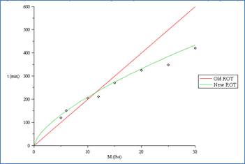
Slightly more practically, they have used Maple to derive a new rule of thumb for the cooking time of turkeys. The traditional rule of thumb is to allow 20 minutes per pound of turkey if you cook at 350° F (after pre-heating to 400° F) although there is a variation to this rule that suggests adding an extra 15 minutes to the final cooking time. According to Maplesoft’s analysis, this is great if your turkey is somewhere between 9 and 14 pounds in weight but if you use it to cook larger turkeys then you may find that the result is overcooked and dry.
After a bit of analysis, Maplesoft have suggested that if the weight of your turkey is x pounds then the ideal cooking time is 45*x^(2/3) minutes. So, using the new rule on a 10 pound turkey gives 45*10^(2/3) = (approx) 209 minutes compared to 200 minutes using the old rule – not much difference there then.
On a 20 pound turkey, however, the difference is more pronounced: 400 minutes using the old rule but 332 minutes using the new rule! Now, the Maple engineer who derived this equation admits that he hasn’t tried it out in the kitchen yet but he will do so this Christmas and I think that I might try it too if I get the chance. If you are a cook and have tried this new formula for large turkeys then let me know how you got on.
Please consider this formula to be experimental for now though and CHECK that your turkey is cooked before eating it. Remember that the equation hasn’t been checked in the kitchen yet!
For more examples of festive mathematical programs created with software such as Mathematica, Maple, MATLAB and SAGE check out the following links.
Earlier this month I had a query from a colleague who had installed MATLAB on some very large and powerful workstations which are used by many researchers at our University. This colleague is a sysadmin of the old school and he doesn’t like installing any program that doesn’t have some sort of validation suite since he wants to be sure that the program is working OK on his hardware for his people to the best of his ability.
He can do this for the NAG library and he can do it for SAGE math (among others) but not, as far as he knew,for MATLAB. So he asked me the question “Does MATLAB have a validation suite?” and since I didn’t have a clue I passed it onto Mathworks Tech support who quickly informed us that the answer was “No.”
The essential gist of the reply was that they assume that MATLAB produces the same results on different machines except, of course, when it doesn’t!
Of course, people such as my colleague feel that ASSUMING that MATLAB produces the same result on different machines is not good enough which is why he wanted a validation suite in the first place. Life is short though and we didn’t pursue it further – partly because we didn’t have an example which proved Mathwork’s assumption wrong.
We do now though!
On a 64bit Windows 7 install of MATLAB 2009b we get the following (incorrect) behaviour:
 p = [1,11-i;2,2;3,3;4,4;5,5;6,6;7,7;8,8;9,9;10,10;11,11];
sort(p)

ans =

   1.0000             2.0000 - 1.0000i
   2.0000             3.0000
   3.0000             4.0000
   4.0000             5.0000
   5.0000             6.0000
   6.0000             7.0000
   7.0000             8.0000
   8.0000             9.0000
   9.0000            10.0000
  10.0000            11.0000
  11.0000            11.0000
On the same machine but booted into 64bit Ubuntu 9.10 we get the correct behaviour:
 p = [1,11-i;2,2;3,3;4,4;5,5;6,6;7,7;8,8;9,9;10,10;11,11];
sort(p)

ans =

   1.0000             2.0000
   2.0000             3.0000
   3.0000             4.0000
   4.0000             5.0000
   5.0000             6.0000
   6.0000             7.0000
   7.0000             8.0000
   8.0000             9.0000
   9.0000            10.0000
  10.0000            11.0000
  11.0000            11.0000 - 1.0000i
Is this exactly the type of bug that might have been caught in a validation suite? Would a user-runnable validation suite be useful?
Thanks to Michal Kvasnicka who alerted me to this bug which was first described in a discussion thread on MATLAB central. Mathworks are aware of the bug and have logged it as issue number 594221.
Picture the scene….
A math instructor and her student are working through a problem together and on the first line it says
f(x) = 2(x+3)
“So” says the instructor “What do we have here?”
The student thinks for a second before replying, “f of x equals 2 of x+3”
The instructor gives a long sigh and puts her head in her hands.
“Have I taught you nothing?” she asks desparingly as the student looks on in bewilderment. Who has the conceptual misunderstanding of this situation; the teacher or the student?
There have been a couple of blog posts recently that have focused on creating interactive demonstrations for the discrete logistic equation – a highly simplified model of population growth that is often used as an example of how chaotic solutions can arise in simple systems. The first blog post over at Division by Zero used the free GeoGebra package to create the demonstration and a follow up post over at MathRecreation used a proprietary package called Fathom (which I have to confess I have never heard of – drop me a line if you have used it and like it). Finally, there is also a Mathematica demonstration of the discrete logistic equation over at the Wolfram Demonstrations project.
I figured that one more demonstration wouldn’t hurt so I coded it up in SAGE – a free open source mathematical package that has a level of power on par with Mathematica or MATLAB. Here’s the code (click here if you’d prefer to download it as a file).
def newpop(m,prevpop):
return m*prevpop*(1-prevpop)
def populationhistory(startpop,m,length):
history = [startpop]
for i in range(length):
history.append( newpop(m,history[i]) )
return history
@interact
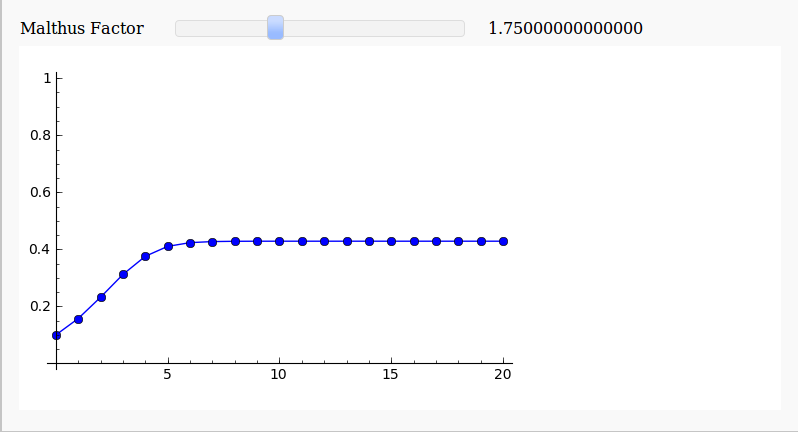
def _( m=slider(0.05,5,0.05,default=1.75,label='Malthus Factor') ):
myplot=list_plot( populationhistory(0.1,m,20) ,plotjoined=True,marker='o',ymin=0,ymax=1)
myplot.show()
Here’s a screenshot for a Malthus Factor of 1.75
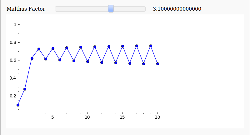
and here’s one for a Malthus Factor of 3.1
There are now so many different ways to easily make interactive mathematical demonstrations that there really is no excuse not to use them.
Update (11th December 2009)
As Harald Schilly points out, you can make a nice fractal out of this by plotting the limit points. My blogging software ruined his code when he placed it in the comments section so I reproduce it here (but he’s also uploaded it to sagenb)
var('x malthus')
step(x,malthus) = malthus * x * (1-x)
stepfast = fast_callable(step, vars=[x, malthus], domain=RDF)

def logistic(m, step):
   # filter cycles
   v = .5
   for i in range(100):
       v = stepfast(v,m)
   points = []
   for i in range(100):
       v = stepfast(v,m)
       points.append((m+step*random(),v))
   return points
points=[]
step = 0.005
for m in sxrange(2.5,4,step):
   points += logistic(m, step)
point(points,pointsize=1).show(dpi=150)

The 60th edition of the Carnival of Mathematics has been posted by Nick Hamblet over at his blog Sumidiot and is a veritable feast of mathematical goodness. Containing some of the very best mathematical blog posts from the last 4 weeks it includes topics as diverse as the symmetry of buckyballs through to Gaussian Primes. There’s also a selection of puzzles (some with solutions and others that have never been solved by anyone), beautiful three dimensional fractals, a case of mistaken identity and infinite trumpets!
If you are one of those people who think that maths is just about manipulating equations or calculating things then prepare for a culture shock!
If one carnival a month simply isn’t enough for you then you are in luck because there is SO MUCH in the mathematical blogsphere that we can put on two shows a month. Math teachers at play (MTAP) is a carnival that has the same spirit as the carnival of maths but is restricted to preK-12 mathematical topics (If, like me, you are from the UK then that means everything up to and including A-Level). The last one was published two weeks ago on November the 20th over at Let’s Play Math and included an astonishing variety of mathematical writing. Denise, the owner of Let’s play math, looks after the administration of MTAP and she’s always looking for new hosts so please do contact her if you are interested.
If, on the other hand, you’d like to host the next carnival of mathematics (due for publication in January) then you need to speak to me and the easiest way to do this is to write a comment to this post. Include your email address with your comments and I’ll get back to you as soon as possible (rest assured that no one but me will see your email address).
I don’t care what level of mathematics you have, from barely being able to count through to a PhD in combinatorics – you simply cannot fail to find something that will amuse, delight and educate you in these carnivals. The mathematical blogging community is not just active, it’s positively fizzing with talented writers, educators, enthusiasts and researchers.
Enjoy!
The student version of MATLAB is a bargain since it only costs $99 (or less than £50 for those of us in the UK) and it comes complete with several toolboxes including symbolic maths, statistics and optimisation. Most of it is identical to the full academic version which would cost well over a thousand pounds if you bought all of the toolboxes included in the student version. The only place where it is ‘crippled’ is within Simulink since your Simulink models are limited to 1000 blocks. There are one or two other differences too and I refer you to the amazon page
for full details (Amazon is also the cheapest place I could find for Student MATLAB by the way).
One problem with the student version of MATLAB though is the fact that they only supply a 32 bit version. This was potentially a big problem for a friend of mine since he has a 64bit Linux machine with 4Gb of RAM. Fortunately, the 32bit version installs OK on 64bit Linux but the result is completely unsupported by Mathworks. Fair enough….It works and he is (mostly) happy since he gets a lot of functionality for his money.
One thing that definitely didn’t work though was compiling mex files. No matter how hard we tried we simply could not get it to work which made me look bad because I am supposed to be ‘The MATLAB guy’ around here. Well, sometimes it’s not what you know but who you know that counts and I know a LOT of MATLAB users. One of them has provided a fix but doesn’t want his name plastered all over Walking Randomly. So, thanks to Mr Anonymous we got mex files working on Student MATLAB 2009a running on 64bit Linux and this is how we did it.
Get a simple mex file and try to compile it. You’ll probably get this error.
/usr/bin/ld: cannot find -lmx
The way to get around that is to run the following command in MATLAB just before you try to compile a mex file
setenv('MATLAB_ARCH', 'glnx86') (IN MATLAB)
That gets you a little further but you’ll next be hit by
/usr/bin/ld: cannot find -lstdc++
To fix this you need to find your mexopts.sh file and change the line
CLIBS="$CLIBS -lstdc++"
to
CLIBS="$CLIBS -L/home/paul/matlab/R2009a-student/sys/os/glnx86 -lstdc++"
obviously, you’ll need to change /home/paul/matlab to wherever you actually installed MATLAB.
Your next step is to do the following in a bash prompt
ln -s /home/paul/matlab/R2009a-student/sys/os/glnx86/libstdc++.so.6 \
/home/paul/matlab/R2009a-student/sys/os/glnx86/libstdc++.so
again – substituting wherever you installed MATLAB for /home/paul/matlab
Paul was running Ubuntu 9.04 and he got the following error at some point (I can’t remember where)
/usr/include/gnu/stubs.h:7:27: error: gnu/stubs-32.h: No such file or directory
which was fixed by
sudo apt-get install libc6-dev-i386
That’s pretty much it. You should now be able to compile mex files. Hope this helps someone out there.