
A faster version of MATLAB’s interp1
I often get sent a piece of code written in something like MATLAB or Mathematica and get asked ‘how can I make this faster?‘. I have no doubt that some of you are thinking that the correct answer is something like ‘completely rewrite it in Fortran or C‘ and if you are then I can only assume that you have never been face to face with a harassed, sleep-deprived researcher who has been sleeping in the lab for 7 days straight in order to get some results prepared for an upcoming conference.
Telling such a person that they should throw their painstakingly put-together piece of code away and learn a considerably more difficult language in order to rewrite the whole thing is unhelpful at best and likely to result in the loss of an eye at worst. I have found that a MUCH better course of action is to profile the code, find out where the slow bit is and then do what you can with that. Often you can get very big speedups in return for only a modest amount of work and as a bonus you get to keep the use of both of your eyes.
Recently I had an email from someone who had profiled her MATLAB code and had found that it was spending a lot of time in the interp1 function. Would it be possible to use the NAG toolbox for MATLAB (which hooks into NAG’s superfast Fortran library) to get her results faster she wondered? Between the two of us and the NAG technical support team we eventually discovered that the answer was a very definite yes.
Rather than use her actual code, which is rather complicated and domain-specific, let’s take a look at a highly simplified version of her problem. Let’s say that you have the following data-set
 x = [0;0.2;0.4;0.6;0.75;0.9;1];
 y = [1;1.22140275816017;1.49182469764127;1.822118800390509;2.117000016612675;2.45960311115695; 2.718281828459045];
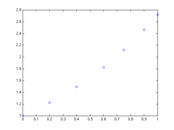
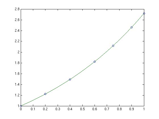
and you want to interpolate this data on a fine grid between x=0 and x=1 using piecewise cubic Hermite interpolation. One way of doing this in MATLAB is to use the interp1 function as follows
tic
t=0:0.00005:1;
y1 = interp1(x,y,t,'pchip');
toc
The tic and toc statements are there simply to provide timing information and on my system the above code took 0.503 seconds. We can do exactly the same calculation using the NAG toolbox for MATLAB:
tic
[d,ifail] = e01be(x,y);
[y2, ifail] = e01bf(x,y,d,t);
toc
which took 0.054958 seconds on my system making it around 9 times faster than the pure MATLAB solution – not bad at all for such a tiny amount of work. Of course y1 and y2 are identical as the following call to norm demonstrates
norm(y1-y2)
ans =
      0
Of course the real code contained a lot more than just a call to interp1 but using the above technique decreased the run time of the user’s application from 1 hour 10 minutes down to only 26 minutes.
Thanks to the NAG technical support team for their assistance with this particular problem and to the postgraduate student who came up with the idea in the first place.
Mike, so you are saying that fitting 7 datapoints takes 0.5 seconds ?! That sounds ridiculous right? I tried doing it in Mathematica, it takes 0.1 second the first time, but after the packages are loaded only milliseconds. And that even includes 2 plots!
AbsoluteTiming[
x={0,0.2,0.4,0.6,0.75,0.9,1};
y={1,1.22140275816017,1.49182469764127,1.822118800390509,2.117000016612675,2.45960311115695,2.718281828459045};
l1=ListPlot[Transpose[{x,y}]];
timesol=Interpolation[Transpose[{x,y}],InterpolationOrder->1, Method->”Hermite”];
p1=Plot[timesol[x],{x,0,1}];
Show[{l1,p1}]
]
So maybe she should give Mathematica a try? What do you think?
Hi Sander
I don’t think that you are comparing like for like. Finding the splines that fit the 7 datapoints is trivial no matter which package you use. Evaluating them at 20001 different points (the length of the vector t in my example) is what takes the time and it was this time that we wanted to minimise. A closer Mathematica equivalent would be
AbsoluteTiming[
 x = {0, 0.2000000, 0.4000000, 0.6000000, 0.75000000, 0.9000000, 1};
 y = {1, 1.22140275816017, 1.49182469764127, 1.822118800390509,
   2.117000016612675, 2.45960311115695, 2.718281828459045};
 timesol = Interpolation[Transpose[{x, y}], Method -> "Hermite"];
 y1 = Table[timesol[x], {x, 0, 1, 0.00005}];
 ]
On the system where I currently sit (different from the one I used when I wrote the article) I get the following timings using the code in the article and the Mathematica code above.
NAG/MATLAB – 0.035 seconds
Mathematica – 0.062 seconds
MATLAB – 0.095 seconds
What I don’t understand here is why my MATLAB score for this system is so much better than my other one since the hardware is almost identical.
NAG is still faster but not as much as I originally thought.
Maybe I need to do more sophicsticated timings than just tic and toc? I will invesitigate.
OK so I should have known better – individual timings can vary wildy and I should have taken an average of many runs. So I did.
x = [0;0.2;0.4;0.6;0.75;0.9;1];
y = [1;1.22140275816017;1.49182469764127;1.822118800390509;2.117000016612675;2.45960311115695; 2.718281828459045];
t=0:0.000005:1;

matlabtimes=zeros(1,100);
nagtimes=zeros(1,100);
for n=1:100
    tic
    [d,ifail] = e01be(x,y);
    [y2, ifail] = e01bf(x,y,d,t);
    nagtimes(n)=toc;
end

for n=1:100
    tic
    y1 = interp1(x,y,t,'pchip');
    matlabtimes(n)=toc;
end
Finding the average times as follows
mean(matlabtimes)

ans =

    0.0390
>> mean(nagtimes)

ans =
    0.0022
So I was wrong. The NAG solution isn’t 9 times faster than the MATLAB version. It’s 17 times faster on average!
Both NAG/MATLAB and pure MATLAB are faster than Mathematica.
Hi Mike,
I enjoy reading your blog.
Your timing of INTERP1 of Matlab surprises me. I assume you use the latest version of Matlab.
I use R2008a on a 6+ years old Dell Precission 450 with Windows XP SP3.
I think that “… individual timings can vary wildy …” is not true regarding Matlab. (Assuming that not other processes are competing for the cpu-cycles.)
Here are a couple of my results.
Execution of your original script:
>> clear all
…
Elapsed time is 0.260425 seconds. — first call – functions are loaded into memory
Elapsed time is 0.048815 seconds. — second call – ???
Elapsed time is 0.011384 seconds.
Elapsed time is 0.009701 seconds.
Elapsed time is 0.009132 seconds.
Elapsed time is 0.009301 seconds.
Elapsed time is 0.008757 seconds.
I repeated this a few time and see the same pattern every time.
Execution two times of the loop. It does not include the assignment of t. Mean and standard deviation of the results of the second run are:
>> mean(matlabtimes)
ans =
0.0082
>> std(matlabtimes)
ans =
6.7250e-004
/ per isakson
Mike,
I didn’t see that, sorry for the quick judging. However don’t use table in Mathematica, it is most often not so fast, there are faster ways:
timesol /@ Range[0, 1, 0.00005]
or even
timesol[Range[0,1,0.00005]] (as the function automatically threads over a list of arguments).
Please try those as well, it could be quite a bit of difference!, and while your at it; please also average over 100 runs ;-)
Sander
Per,
You are right – it seems that it’s only the first run that is much different from the others. I’m using 2009a on Windows XP SP3. Would you mind running the following please (the one in the comment above) It has a larger t and is repeated 100 times just to make sure?
x = [0;0.2;0.4;0.6;0.75;0.9;1]; y = [1;1.22140275816017;1.49182469764127;1.822118800390509;2.117000016612675;2.45960311115695; 2.718281828459045]; t=0:0.000005:1; matlabtimes=zeros(1,100); for n=1:100 tic y1 = interp1(x,y,t,'pchip'); matlabtimes(n)=toc; end mean(matlabtimes)Sander,
Table is slow? First I’ve heard about it! I remember back in the day being told ‘Don’t use Do loops – use Table because it’s faster’. Thanks for letting me know – as soon as I get into uni tomorrow I’ll check it out. Might be another blog post in that.
Cheers,
Mike
Mike,
I often try to circumvent using table, but rather using Map (/@). Note that Table is not always slower, it is sometimes faster than Map. But if you have a list of values, and you want to evaluate a function at those values, most often Map (/@) is the fastest. It just depends on the task which is faster, I often try both with varying result.
I think in general you can say: For < Table and in some cases For < Table < Map.
This code finds the first n primes as a list, it can be done in many, many ways, here are a couple:
n=600000;
t1=AbsoluteTiming[Prime[Range[1,n]];];
t2=AbsoluteTiming[Prime/@Range[1,n];];
t3=AbsoluteTiming[Map[Prime,Range[1,n]];];
t4=AbsoluteTiming[Table[Prime[x],{x,1,n}];];
t5=AbsoluteTiming[Reap[Do[Sow[Prime[i]],{i,1,n}]][[2,1]];];
t6=AbsoluteTiming[res=ConstantArray[0,n];Do[res[[i]]=Prime[i],{i,1,n}];];
t7=AbsoluteTiming[Reap[For[i=1,i<=n,i++,Sow[Prime[i]]]][[2,1]];];
t8=AbsoluteTiming[res=ConstantArray[0,n];For[i=1,i<=n,i++,res[[i]]=Prime[i]];];
times={t1,t2,t3,t4,t5,t6,t7,t8}[[All,1]]
BarChart[times]
Sometimes it is worth looking in to the way you make a list!
Sander
Counterexample when Table is faster than Map could be the simple task of adding 2:
AbsoluteTiming[# + 2 & /@ Range[10^6];]
AbsoluteTiming[Table[i + 2, {i, 10^6}];]
(note that Range[10^6)+2 is way faster, or one could even type Range[3,10^6+2], which is again much faster)
Cheers,
Sander
An example where Map is faster than Table would be
AbsoluteTiming[Table[PrimeQ[i], {i, 0, 10000000}];]
AbsoluteTiming[PrimeQ /@ Range[0, 10000000];]
On my computer the latter is about 7.5% faster. Not a lot, but it’s something :-)
Ok, last comment of the day!
Sander
Mike,
Now, I have run the loop with the larger t (0.2e6 elements, numel(t)=200001 ). It takes 10 times longer. In this case, function or script doesn’t affect the speed – I checked. (The JIT-compiler used to be more effective with functions.)
>> clear all
mean = 0.0858, std = 0.0257
mean = 0.0824, std = 0.0015
/ per
Thanks for that per – your results are in line with mine considering your computers speed etc. I guess that the time I mentioned in the post was an anomaly which could have rendered the whole post pointless but fortunatley for me everything checks out just fine. Just to repeat I get the following times using the script that you have just tried.
MATLAB interp1 – 0.0390 seconds
NAG – 0.0022 seconds
So the NAG result is 17 times faster.
Thanks for all the feedback – I’ll be more careful in future :)
I never trust numerical “benchmark” demonstrations that take less than a second to run, much less those that take a fraction of a second. There could be too much stuff going on in the background. If you want to benchmark something, write a loop that does the same thing over and over, close all applications, let it run for several minutes.
I do believe that NAG should be much faster. A lot of Matlab functions are written in Matlab’s language, but NAG library is compiled code. Now, if only my university had a license for NAG. It would be interesting to see how much faster is NAG’s optimization code, arma estimation, and other statistical routines. I suspect much fast since most of this code in Matlab’s toolboxes is based on interpreted m-files. This is specially bad for optimization routines, most of which have to run in a loop.
Hi Jacob
We did do it in a loop and took an average. The code used was
x = [0;0.2;0.4;0.6;0.75;0.9;1];
y = [1;1.22140275816017;1.49182469764127;1.822118800390509;2.117000016612675;2.45960311115695; 2.718281828459045];
t=0:0.000005:1;

matlabtimes=zeros(1,100);
for n=1:100
    tic
    y1 = interp1(x,y,t,'pchip');
    matlabtimes(n)=toc;
end
mean(matlabtimes)
As for other NAG functions – I imagine that some will be faster than MATLAB whereas other won’t be. MATLAB uses compiled code too for certain functions and it will be here where NAG’s advantage might go away.
I don’t intend on working through a systematic set of benchmarks for lots of functions. If I find a production MATLAB code that needs speeding up where I can drop in a NAG function then I’ll try it out.
Cheers,
Mike
Oh, I am sorry. I did not intend to ask you to benchmark anything. I just wondered, in general, how much, if at all, NAG functions could be faster than the MATLAB implementations for doing statistical work in things like say time series analysis. I am almost certain that NAG will be faster since probably all of NAG is compiled code but only some of MATLAB’s functions are compiled into libraries. For example, Matlab’s ARMA-GARCH family of functions in econometrics toolbox seems to be written entirely as MATLAB scripts, as well as many things in the optimization toolbox. I believe there is a general view in the statistics community that MATLAB’s optimization is weaker than other packages, but I don’t know to what extent this is true. When I have time, I’ll download the trial copy of NAG toolbox to try it myself.
Hi Jacob
No worries. I actually would be interested in collaborating with someone to do a small selection of benchmarks so feel free to get in touch if you’d like to work through something. I don’t want to do a thorough study of 100s of functions but concentrating on a small subset of commonly used functions might result in something useful.
Cheers,
Mike