Walking Randomly

There are lots of Widgets in ipywidgets. Here’s how to list them

from ipywidgets import *
widget.Widget.widget_types

At the time of writing, this gave me

{'Jupyter.Accordion': ipywidgets.widgets.widget_selectioncontainer.Accordion,
 'Jupyter.BoundedFloatText': ipywidgets.widgets.widget_float.BoundedFloatText,
 'Jupyter.BoundedIntText': ipywidgets.widgets.widget_int.BoundedIntText,
 'Jupyter.Box': ipywidgets.widgets.widget_box.Box,
 'Jupyter.Button': ipywidgets.widgets.widget_button.Button,
 'Jupyter.Checkbox': ipywidgets.widgets.widget_bool.Checkbox,
 'Jupyter.ColorPicker': ipywidgets.widgets.widget_color.ColorPicker,
 'Jupyter.Controller': ipywidgets.widgets.widget_controller.Controller,
 'Jupyter.ControllerAxis': ipywidgets.widgets.widget_controller.Axis,
 'Jupyter.ControllerButton': ipywidgets.widgets.widget_controller.Button,
 'Jupyter.Dropdown': ipywidgets.widgets.widget_selection.Dropdown,
 'Jupyter.FlexBox': ipywidgets.widgets.widget_box.FlexBox,
 'Jupyter.FloatProgress': ipywidgets.widgets.widget_float.FloatProgress,
 'Jupyter.FloatRangeSlider': ipywidgets.widgets.widget_float.FloatRangeSlider,
 'Jupyter.FloatSlider': ipywidgets.widgets.widget_float.FloatSlider,
 'Jupyter.FloatText': ipywidgets.widgets.widget_float.FloatText,
 'Jupyter.HTML': ipywidgets.widgets.widget_string.HTML,
 'Jupyter.Image': ipywidgets.widgets.widget_image.Image,
 'Jupyter.IntProgress': ipywidgets.widgets.widget_int.IntProgress,
 'Jupyter.IntRangeSlider': ipywidgets.widgets.widget_int.IntRangeSlider,
 'Jupyter.IntSlider': ipywidgets.widgets.widget_int.IntSlider,
 'Jupyter.IntText': ipywidgets.widgets.widget_int.IntText,
 'Jupyter.Label': ipywidgets.widgets.widget_string.Label,
 'Jupyter.PlaceProxy': ipywidgets.widgets.widget_box.PlaceProxy,
 'Jupyter.Play': ipywidgets.widgets.widget_int.Play,
 'Jupyter.Proxy': ipywidgets.widgets.widget_box.Proxy,
 'Jupyter.RadioButtons': ipywidgets.widgets.widget_selection.RadioButtons,
 'Jupyter.Select': ipywidgets.widgets.widget_selection.Select,
 'Jupyter.SelectMultiple': ipywidgets.widgets.widget_selection.SelectMultiple,
 'Jupyter.SelectionSlider': ipywidgets.widgets.widget_selection.SelectionSlider,
 'Jupyter.Tab': ipywidgets.widgets.widget_selectioncontainer.Tab,
 'Jupyter.Text': ipywidgets.widgets.widget_string.Text,
 'Jupyter.Textarea': ipywidgets.widgets.widget_string.Textarea,
 'Jupyter.ToggleButton': ipywidgets.widgets.widget_bool.ToggleButton,
 'Jupyter.ToggleButtons': ipywidgets.widgets.widget_selection.ToggleButtons,
 'Jupyter.Valid': ipywidgets.widgets.widget_bool.Valid,
 'jupyter.DirectionalLink': ipywidgets.widgets.widget_link.DirectionalLink,
 'jupyter.Link': ipywidgets.widgets.widget_link.Link}

I was in a funk!

Not long after joining the University of Sheffield, I had helped convince a raft of lecturers to switch to using the Jupyter notebook for their lecturing. It was an easy piece of salesmanship and a whole lot of fun to do. Lots of people were excited by the possibilities.

The problem was that the University managed desktop was incapable of supporting an instance of the notebook with all of the bells and whistles included. As a cohort, we needed support for Python 2 and 3 kernels as well as R and even Julia. The R install needed dozens of packages and support for bioconductor. We needed LateX support to allow export to pdf and so on. We also needed to keep up to date because Jupyter development moves pretty fast! When all of this was fed into the managed desktop packaging machinery, it died. They could give us a limited, basic install but not one with batteries included.

I wanted those batteries!

In the early days, I resorted to strange stuff to get through the classes but it wasn’t sustainable. I needed a miracle to help me deliver some of the promises I had made.

Miracle delivered – SageMathCloud

During the kick-off meeting of the OpenDreamKit project, someone introduced SageMathCloud to the group. This thing had everything I needed and then some! During that presentation, I could see that SageMathCloud would solve all of our deployment woes as well as providing some very cool stuff that simply wasn’t available elsewhere. One killer-application, for example, was Google-docs-like collaborative editing of Jupyter notebooks.

I fired off a couple of emails to the lecturers I was supporting (“Everything’s going to be fine! Trust me!”) and started to learn how to use the system to support a course. I fired off dozens of emails to SageMathCloud’s excellent support team and started working with Dr Marta Milo on getting her Bioinformatics course material ready to go.

TL; DR: The course was a great success and a huge part of that success was the SageMathCloud platform

Giving back – A tutorial for lecturers on using SageMathCloud

I’m currently working on a tutorial for lecturers and teachers on how to use SageMathCloud to support a course. The material is licensed CC-BY and is available at https://github.com/mikecroucher/SMC_tutorial 

If you find it useful, please let me know. Comments and Pull Requests are welcome.

If you have an interest in mathematics, you’ve almost certainly stumbled across The Wolfram Demonstrations Project at some time or other.  Based upon Wolfram Research’s proprietary Mathematica software and containing over 8000 interactive demonstrations, The Wolfram Demonstrations Project is a fantastic resource for anyone interested in mathematics and related sciences; and now it has some competition.

Sage is a free, open source alternative to software such as Mathematica and, thanks to its interact function, it is fully capable of producing advanced, interactive mathematical demonstrations with just a few lines of code.  The Sage language is based on Python and is incredibly easy to learn.

The Sage Interactive Database has been launched to showcase this functionality and its looking great.  There’s currently only 31 demonstrations available but, since anyone can sign up and contribute, I expect this number to increase rapidly.  For example, I took the simple applet I created back in 2009 and had it up on the database in less than 10 minutes!  Unlike the Wolfram Demonstrations Project, you don’t need to purchase an expensive piece of software before you can start writing Sage Interactions….Sage is free to everyone.

Not everything is perfect, however.  For example, there is no native Windows version of Sage.  Windows users have to make use of a Virtualbox virtual machine which puts off many people from trying this great piece of software.  Furthermore, the interactive ‘applets’ produced from Sage’s interact function are not as smooth running as those produced by Mathematica’s Manipulate function.  Finally, Sage’s interact doesn’t have as many control options as Mathematica’s Manipulate (There’s no Locator control for example and my bounty still stands).

The Sage Interactive Database is a great new project and I encourage all of you to head over there, take a look around and maybe contribute something.

Regular readers of Walking Randomly will know that I am a big fan of the Manipulate function in Mathematica.  Manipulate allows you to easily create interactive mathematical demonstrations for teaching, research or just plain fun and is the basis of the incredibly popular Wolfram Demonstrations Project.

Sage, probably the best open source mathematics software available right now, has a similar function called interact and I have been playing with it a bit recently (see here and here) along with some other math bloggers.  The Sage team have done a fantastic job with the interact function but it is missing a major piece of functionality in my humble opinion – a Locator control.

In Mathematica the default control for Manipulate is a slider:

Manipulate[Plot[Sin[n x], {x, -Pi, Pi}], {n, 1, 10}]

The slider is also the default control for Sage’s interact:

@interact
def _(n=(1,10)):
    plt=plot(sin(n*x),(x,-pi,pi))
    show(plt)

Both systems allow the user to use other controls such as text boxes, checkboxes and dropdown menus but Mathematica has a control called a Locator that Sage is missing.  Locator controls allow you to directly interact with a plot or graphic.  For example, the following Mathematica code (taken from its help system) draws a polygon and allows the user to click and drag the control points to change its shape.

Manipulate[Graphics[Polygon[pts], PlotRange -> 1],
 {{pts, {{0, 0}, {.5, 0}, {0, .5}}}, Locator}]

The Locator control has several useful options that allow you to customise your demonstration even further. For example, perhaps you want to allow the user to move the vertices of the polygon but you don’t want them to be able to actually see the control points. No problem, just add Appearance -> None to your code and you’ll get what you want.

Manipulate[Graphics[Polygon[pts], PlotRange -> 1],
 {{pts, {{0, 0}, {.5, 0}, {0, .5}}}, Locator, Appearance -> None}]

Another useful option is LocatorAutoCreate -> True which allows the user to create extra control points by holding down CTRL and ALT (or just ALT – it depends on your system it seems) as they click in the active area.

Manipulate[Graphics[Polygon[pts], PlotRange -> 1],
 {{pts, {{0, 0}, {.5, 0}, {0, .5}}}, Locator,
  LocatorAutoCreate -> True}]

When you add all of this functionality together you can do some very cool stuff with just a few lines of code. Theodore Gray’s curve fitting code on the Wolfram Demonstrations project is a perfect example.

All of these features are demonstrated in the video below

So, onto the bounty hunt.  I am offering 25 pounds worth (about 40 American Dollars) of books from Amazon to anyone who writes the code to implement a Locator control for Sage’s interact function.  To get the prize your code must fulfil the following spec

• Your code must be accepted into the Sage codebase and become part of the standard install.  This should ensure that it is of reasonable quality.
• There should be an option like Mathematica’s LocatorAutoCreate -> True to allow the user to create new locator points interactively by Alt-clicking (or via some other suitable method).
• There should be an option to alter the appearance of the Locator control (e.g. equivalent to Mathematica’s Appearance -> x option).  As a minimum you should be able to do something like Appearance->None
• You should provide demonstration code that implements everything shown in the video above.
• I have to be happy with it!

And the details of the prize:

• I only have one prize – 25 pounds worth of books (about 40 American dollars) from Amazon.  If more than one person claims it then the prize will be split.
• The 25 pounds includes whatever it will cost for postage and packing.
• I won’t send you the voucher – I will send you the books of your choice as a ‘gift’.  This will mean that you’ll have to send me your postal address. Don’t enter if this bothers you for some reason.
• I expect you to be sensible regarding the exact value of the prize.  So if your books come to 24.50 then we’ll call it even.  Similarly if they come to 25.50 then I won’t argue.
• I am not doing this on behalf of any organisation.  It’s my personal money.
• My decision is final and I can withdraw this prize offer at any time without explanation.  I hope you realise that I am just covering my back by saying this – I have every intention of giving the prize but whenever money is involved one always worries about the possibility of being ripped off.

Good luck!

Update (29th December 2009): The bounty hunt has only been going for a few days and the bounty has already doubled to 50 pounds which is around 80 American dollars.  Thanks to David Jones for his generosity.

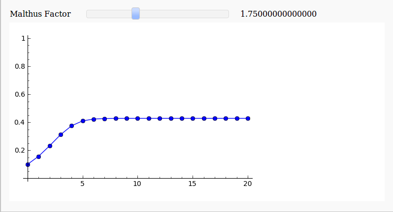
There have been a couple of blog posts recently that have focused on creating interactive demonstrations for the discrete logistic equation – a highly simplified model of population growth that is often used as an example of how chaotic solutions can arise in simple systems.  The first blog post over at Division by Zero used the free GeoGebra package to create the demonstration and a follow up post over at MathRecreation used a proprietary package called Fathom (which I have to confess I have never heard of – drop me a line if you have used it and like it).  Finally, there is also a Mathematica demonstration of the discrete logistic equation over at the Wolfram Demonstrations project.

I figured that one more demonstration wouldn’t hurt so I coded it up in SAGE – a free open source mathematical package that has a level of power on par with Mathematica or MATLAB.  Here’s the code (click here if you’d prefer to download it as a file).

def newpop(m,prevpop):
    return m*prevpop*(1-prevpop)

def populationhistory(startpop,m,length):
    history = [startpop]
    for i in range(length):
        history.append( newpop(m,history[i]) )
    return history

@interact
def _( m=slider(0.05,5,0.05,default=1.75,label='Malthus Factor') ):
    myplot=list_plot( populationhistory(0.1,m,20) ,plotjoined=True,marker='o',ymin=0,ymax=1)
    myplot.show()

Here’s a screenshot for a Malthus Factor of 1.75

and here’s one for a Malthus Factor of 3.1

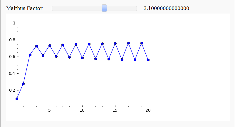
There are now so many different ways to easily make interactive mathematical demonstrations that there really is no excuse not to use them.

Update (11th December 2009)

As Harald Schilly points out, you can make a nice fractal out of this by plotting the limit points.  My blogging software ruined his code when he placed it in the comments section so I reproduce it here (but he’s also uploaded it to sagenb)

var('x malthus')
step(x,malthus) = malthus * x * (1-x)
stepfast = fast_callable(step, vars=[x, malthus], domain=RDF)

def logistic(m, step):
   # filter cycles
   v = .5
   for i in range(100):
       v = stepfast(v,m)
   points = []
   for i in range(100):
       v = stepfast(v,m)
       points.append((m+step*random(),v))
   return points

points=[]
step = 0.005
for m in sxrange(2.5,4,step):
   points += logistic(m, step)
point(points,pointsize=1).show(dpi=150)

Earlier today I was chatting to a lecturer over coffee about various mathematical packages that he might use for an upcoming Masters course  (note – offer me food or drink and I’m happy to talk about pretty much anything). He was mainly interested in Mathematica and so we spent most of our time discussing that but it is part of my job to make sure that he considers all of the alternatives – both commercial and open source. The course he was planning on running (which I’ll keep to myself out of respect for his confidentiality) was definitely a good fit for Mathematica but I felt that SAGE might suite him nicely as well.

“Does it have nice, interactive functionality like Mathematica’s Manipulate function?” he asked

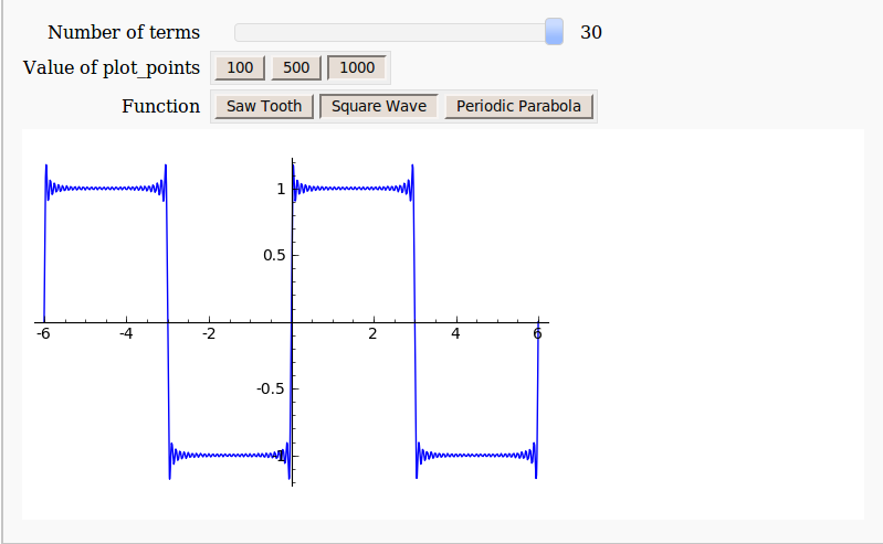
Oh yes! Here is a toy example that I coded up in about the same amount of time that it took to write the introductory paragraph above (but hopefully it has no mistakes). With just a bit of effort pretty much anyone can make fully interactive mathematical demonstrations using completely free software. For more examples of SAGE’s interactive functionality check out their wiki.

Here’s the code:

def ftermSquare(n):
 return(1/n*sin(n*x*pi/3))

def ftermSawtooth(n):
 return(1/n*sin(n*x*pi/3))

def ftermParabola(n):
 return((-1)^n/n^2 * cos(n*x))

def fseriesSquare(n):
 return(4/pi*sum(ftermSquare(i) for i in range (1,2*n,2)))

def fseriesSawtooth(n):
 return(1/2-1/pi*sum(ftermSawtooth(i) for i in range (1,n)))

def fseriesParabola(n):
 return(pi^2/3 + 4*sum(ftermParabola(i) for i in range(1,n)))

@interact
def plotFourier(n=slider(1, 30,1,10,'Number of terms')
,plotpoints=('Value of plot_points',[100,500,1000]),Function=['Saw Tooth','Square Wave','Periodic Parabola']):
    if Function=='Saw Tooth':
     show(plot(fseriesSawtooth(n),x,-6,6,plot_points=plotpoints))
    if Function=='Square Wave':
     show(plot(fseriesSquare(n),x,-6,6,plot_points=plotpoints))
    if Function=='Periodic Parabola':
     show(plot(fseriesParabola(n),x,-6,6,plot_points=plotpoints))

My favourite free mathematics package has seen yet another relase. Released back on Thursday June 9th, version 4.1 of SAGE Math includes a nice array of new features, speed-ups and bug-fixes. Head over to the version 4.1 release tour for more details.

One of the things that I like about each new release of SAGE is that there is always something for everyone – no matter what their level of mathematics. For example, release 4.1 includes advanced functionality for constructing elliptic curves and also adds support for constructing irreducible representations of the symmetric group. On the other hand it also includes some new Sudoku solvers, faster integer division and improved histograms.

If you are a user of SAGE then feel free to say hi in the comments section and let me know what you use it for.

While catching up on all of the news I missed while on Vacation, I discovered that the world’s best open-source Maths package saw a new release at the end of May.  I haven’t had chance to download it yet but the breadth and depth of new features is astonishing.  Check out the comprehensive feature-tour here (note to commercial software developers I have bugged in the past – when I say that I’d like a detailed change-log for your latest release, this is the kind if thing I mean).

Scanning through the changes I note that they have dropped Maxima for core symbolic manipulation in favour of a package called Pynac.   Apparently, one practical upshot of this is that finding the determinant of symbolic matrices can be up to 2500 times faster!  very impressive.  I wonder how this change will affect symbolic calculus (if at all).

Unfortunately,  it looks like a full, native Windows version is still some way off which is a shame because one of my jobs this month is to prepare a load of maths applications for deployment on my University’s teaching clusters which run Windows.  Putting SAGE next to Mathematica, MATLAB and Mathcad would have been cool and a great way to encourage undergraduate users at Manchester University to try out the software.

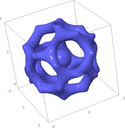
Finally, some eye candy shamelessly stolen from the SAGE website.  The plot below demonstrates the new implicit_plot3d function.

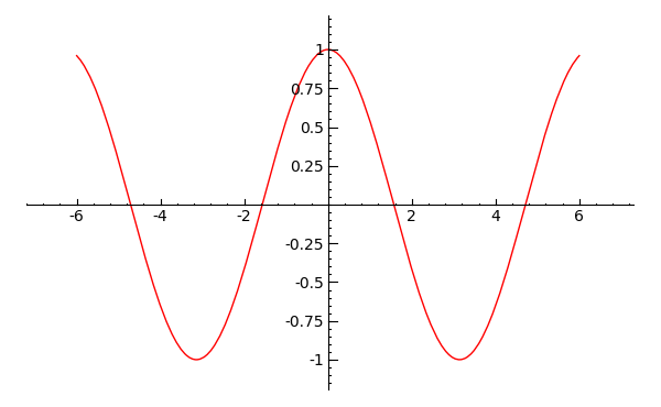
SAGE math is probably the best open-source maths package out there at the moment and slowly but surely I have been learning some of its tricks.  Combining 2D Plots is particularly easy for example.  Let’s plot a cosine curve in red

p1=plot(cos(x),x,-6,6,rgbcolor='red')
show(p1)

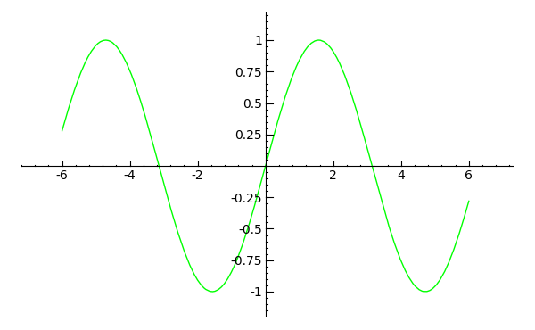
Now let’s plot a sine curve in green

p2=plot(sin(x),x,-6,6,rgbcolor='green')
show(p2)

Combining these two plots into one single plot is extremely intuitive – just add them together

show(p1+p2)

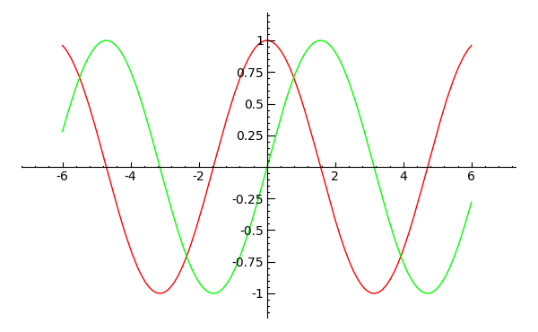
You don’t get much easier than that.  Powerful, easy to use and free – loving it!

The latest version of the powerful free, open-source maths package, SAGE, was released last week.  Version 3.4.1 brings us a lot of new functionality compared to 3.4 and the SAGE team have prepared a detailed document showing us why the upgrade is worthwhile.

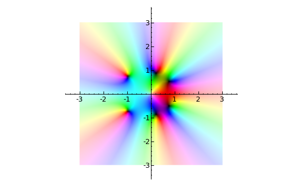
For example, the new complex_plot function looks fantastic.  From the documentation:

The function complex_plot() takes a complex function f(z) of one variable and plots output of the function over the specified xrange and yrange. The magnitude of the output is indicated by the brightness (with zero being black and infinity being white), while the argument is represented by the hue with red being positive real and increasing through orange, yellow, etc. as the argument increases.

sage: f(z) = z^5 + z - 1 + 1/z
sage: complex_plot(f, (-3, 3), (-3, 3))

Sage aims to become a ‘viable free open source alternative to Magma, Maple, Mathematica and Matlab’ and I think it is well on the way.  I become a little more impressed with it with every release and I am a hardcore Mathematica and MATLAB fan.

One major problem with it (IMHO at least) is that there is no native windows version which prevents a lot of casual users from trying it out.  Although you can get it working on Windows, it is far from ideal because you have to run a virtual machine image using VMWare player.  The hard-core techno geeks among you might well be thinking ‘So what?  Sounds easy enough.’ but it’s an extra level of complexity that casual users simply do not want to have to concern themselves with.  Of course there is also the issue of performance – emulating an entire machine to run a single application is hardly a good use of compute resources.

There is a good reason why SAGE doesn’t have a proper Windows version yet – it’s based upon a lot of component parts that don’t have Windows versions and someone has to port each and every one of them.  It’s going to be a lot of work but I think it will be worth it.

When the SAGE development team release a native Windows version of their software then I have no doubt that it will make a significant impact on the mathematical software scene – especially in education.  There will be nothing preventing every school and university in the world from having access to a world-class computer algebra system.

In an ideal world everyone would be running Linux but we don’t live in an ideal world so a Windows version of SAGE would be a step in the right direction.

Update: It turns out that a Windows port is being developed and something should be ready soon – http://windows.sagemath.org/ Thanks to mvngu in the comments section for pointing this out. I should have done my research better!