
Archive for the ‘parallel programming’ Category
The Meltdown bug which affects most modern CPUs has been called by some ‘The worst ever CPU bug’. Accessible explanations about what the Meltdown bug actually is are available here and here.
Software patches have been made available but some people have estimated a performance hit of up to 30% in some cases. Some of us in the High Performance Computing (HPC) community (See here for the initial twitter conversation) started to wonder what this might mean for the type of workloads that run on our systems. After all, if the worst case scenario of 30% is the norm, it will drastically affect the power of our systems and hence reduce the amount of science we are able to support.
In the video below, Professor Mark Handley from University College London gives a detailed explanation of both Meltdown and Spectre at an event held at Alan Turing Institute in London.
Another video that gives a great introduction to this topic was given by Jon Masters at https://fosdem.org/2018/schedule/event/closing_keynote/
To patch or not to patch
To a first approximation, a patch causing a 30% performance hit on a system costing £1 million pounds is going to cost an equivalent of £300,000 — not exactly small change! This has led to some people wondering if we should patch HPC systems at all:
Given the size of the performance hit should we even *be* patching for this? Unless you need trusted computing, does it really matter for the average HPC?
— Phil Tooley (@acceleratedsci) January 5, 2018
All of the UK Tier-3 HPC centres I’m aware of have applied the patches (Sheffield, Leeds and Manchester) but I’d be interested to learn of centres that decided not to. Feel free to comment here or message me on twitter if you have something to add to this discussion and I’ll update this post where appropriate.
Research paper discussing the performance penalties of these patches on HPC workloads
A group of people have written a paper on Arxiv that looks at HPC performance penalties in more detail. From the paper’s abstract:
The results show that although some specific functions can have execution times decreased by as much as 74%, the majority of individual metrics indicates little to no decrease in performance. The real-world applications show a 2-3% decrease in performance for single node jobs and a 5-11% decrease for parallel multi node jobs.
Other relevant results and benchmarks
Here are a few other links that discuss the performance penalty of applying the Meltdown patch.
- Redhat’s experiments showing worst-case performance drops of 19% in certain benchmarks.
- Wikipedia article showing a summary of various benchmarks.
Acknowledgements
Thanks to Adrian Jackson, Phil Tooley, Filippo Spiga and members of the UK HPC-SIG for useful discussions.
UK to launch 6 major HPC centres
Tomorrow, I’ll be attending the launch event for the UK’s new HPC centres and have been asked to deliver a short talk as part of the program. As someone who paddles in the shallow-end of the HPC pool I find this both flattering and more than a little terrifying. What can little-ole-me say to the national HPC glitterati that might be useful?
This blog post is an attempt at gathering my thoughts together for that talk.
The technology gap in research computing
Broadly speaking, my role in academia is to hang out with researchers, compute providers (cloud and HPC) and software vendors in an attempt to be vaguely useful in the area of research software. I’m a Research Software Engineer with a focus on Long Tail Science: The large number of very small research groups who do a huge amount of modern research.
Time and again, what I see can be summarized in this quote by Greg Wilson
This is very true in the world of High Performance Computing.
Geek Top Gear
I love technology and I love HPC in particular. I love to geek out on Flops, Ghz, SIMD instructions, GPUs, FPGAs…..all that stuff. I help support The University of Sheffield’s local HPC service and worked in Research IT at The University of Manchester for around a decade before moving to Sheffield.
I’ve given and seen many a HPC-related talk in my time and have certainly been guilty of delivering what I now refer to as the ‘Geek Top Gear’ speech. For maximum effect, you need to do it in a Jeremy Clarkson voice and, if you’re feeling really macho, kiss your bicep at the point where you tell the audience how many Petaflops your system can do in Linpack.
*Begin Jeremy Clarkson Impression*
Our new HPC system has got 100,000 of the latest Intel Kaby Lake cores...which is a lot!
Usually running at 2.6Ghz, these cores can turbo-boost to 3.2Ghz for those moments when we need that extra boost of power. Obviously, being Kaby Lake, these cores have all the instruction extensions you’d expect with AVX2, FMA, SSE, ABM and many many other TLAs for all your SIMD needs. Of course every HPC system needs accelerators…..and we have the best of them: Xeon Phis with 68 cores each and NVIDIA GPUs with thousands of tiny little cores will handle every massively parallel job you can throw at them….Easily. We connect these many many cores together with high-speed interconnect fashioned from threads of pure unicorn hair and cool the whole thing with the tears of virigin nerds.
YEEEEEES! Our new HPC system is the best one since the last one and, achieving over a Gajillion Petaflops in the Linpack test (kiss bicep), it will change your life forever.

Any questions?
Audience member 1: What’s a core?
Audience member 2: Why does it run my R script slower than my laptop?
Audience member 3: Do you have Excel installed on it?
There is a huge gap between what many HPC providers like to focus on and what the typical long-tail researcher wants or needs. I propose that the best bridge for this gap is the Research Software Engineer (RSE).
Research Software Engineer as Alpine guide
In my fellowship proposal, I compared the role of a Research Software Engineer to that of an alpine guide:
Technological development in software is more like a cliff-face than a ladder – there are many routes to the top, to a solution. Further, the cliff face is dynamic – constantly and quickly changing as new technologies emerge and decline. Determining which technologies to deploy and how best to deploy them is in itself a specialist domain, with many features of traditional research.
Researchers need empowerment and training to give them confidence with the available equipment and the challenges they face. This role, akin to that of an Alpine guide, involves support, guidance, and load carrying. When optimally performed it results in a researcher who knows what challenges they can attack alone, and where they need appropriate support. Guides can help decide whether to exploit well-trodden paths or explore new possibilities as they navigate through this dynamic environment.
At Sheffield, we have built a pool of these Research Software Engineers to provide exactly this kind of support and it’s working extremely well so far. Not only are we helping individual research groups but we are also using our experiences in the field to help shape the University HPC environment in collaboration with the IT department.
Supercomputing: Irrelevant to many?
“Never bring an anecdote to a data-fight” so the saying goes and all I have from my own experiences are a bucket load of anecdotes, case studies and cursory log-mining experiments that indicate that even those who DO use HPC are not doing so effectively. Fortunately, others have stepped up to the plate and we have survey and interview data on how researchers are using compute resources.
How Do Scientists Develop and Use Scientific Software? is a report on a 2009 survey of 1972 researchers from around the world. They found that “79.9% of the scientists never use scientific software on a supercomputer”
When I first learned of this number, I found it faintly depressing. This technology that I love so much and for which University IT departments dedicate special days to seems to be pretty much irrelevant to the majority of researchers. Could it be that even in an era of big data, machine learning and research software engineering that most people only need a laptop?
Only ever needing a laptop certainly doesn’t fit with what I’ve seen while working in the trenches. Almost every researcher I’ve met who does computational research wishes it was faster or that they had more memory to allow them to do larger problems. Speed is the easiest thing to sell to researchers in the world of RSE. They come for faster execution and leave with a side-order of version control, testing and documentation. A combination of software development and migration to even a small HPC system can easily result in 100x or even 1000x speed-ups for many researchers.
In my experience, it’s not that researchers don’t need HPC, it’s that the jump from their laptop-based workflow to one that makes good use of a HPC system is too large for them to bridge without a little help. Providing that help can result in some great partnerships such as the recent one between the Sheffield RSE group and the Sheffield Faculty of Arts and Humanities.

Want to know how that partnership started? I compiled an experimental R/Rcpp package that they were struggling with and then took them for coffee and said ‘That code took a while to run. Here’s how we can make it go faster….Now…what exactly are you doing because it looks cool?’ Fast forward a year or so and we are on the cusp of starting a great new project that will include traditional HPC and cloud computing as part of their R-based workflow.
My experiences seem to be reflected in the data. In their 2011 article, A Survey of the Practice of Computational Science, Prabhu et al interviewed 114 randomly selected researchers from Princeton University. Princeton have a very strong, well supported HPC centre which provides both resources and the expertise to use them. Even at such a well equipped institution, the authors write that ‘Despite enormous wait times, many scientists run their programs only on desktops’ although they did report much higher HPC usage compared to the Hanny et al survey.
Other salient quotes from the Prabhu interviews include
“only 18% of researchers who optimize code leveraged profiling tools to inform their optimization plans”
“only 7% of researchers leveraged any form of thread based shared memory CPU parallelism”
“Only 11% of researchers utilized loop based parallelism”
“Currently, many researchers fit their scientific models to only a subset of available parameters for faster program runs.”
“Across disciplines, an order of magnitude performance improvement was cited as a requirement for significant changes in research quality”
HPC: There’s plenty of room at the bottom
Potential users of HPC look different to those of 20 years ago. The popularity explosion of languages such as MATLAB, Python and R have democratized programming and the world is awash with inefficient research software. Most of the time, this lack of efficiency is not a problem (see ‘In defense of inefficient scientific code‘) but if a researcher needs to scale up what they are doing, it can become limiting. Researchers might wait for days for the results to come in and limit the scope of their investigations to fit the hardware they have access to — their laptop usually.
The paper of Prabu et al said that an order of magnitude (10x) speed up was cited by researchers as a requirement for significant changes in research quality. For an experienced Research Software Engineer with access to cloud or HPC facilities, a 10x speed-up is usually pretty easy to achieve for this new audience. 100x or even 1000x can be achieved fairly frequently if you employ multiple hardware and software techniques. Compared to squeezing out a few percent more performance from HPC-centric code such as LAPACK or CASTEP, it’s not even all that difficult. I recently sped up one researcher’s MATLAB code by a factor of 800x in a couple of days and I’m a fairly middling developer if I’m brutally honest.
The whole point of High Performance Computing is to accelerate science and right now there is more computational science around than there has ever been before. Furthermore, it’s easier than ever to accelerate! There’s plenty of room at the bottom.
Closing the computational gap with people, training and compute power
The UK’s 6 new HPC centers represent the cutting edge of hardware technology. They provide a crucial component of our national hardware infrastructure, will contribute to research in HPC itself and will doubtless be of huge benefit to computational science. Furthermore, all of the funded proposals include significant engagement with the national Research Software Engineering community – the vital bridge between many researchers and HPC.
Co-development of research software with effort from both RSEs and researchers can be an extremely powerful model. Combine this with further collaboration between RSEs and compute providers and we have an environment that I think is both very exciting and capable of helping to close the rich/poor compute divide.
As an RSE who works with both researchers and University-level HPC providers, I ask for 3 things to be considered by these new regional centres.
- Enjoy your new compute-ferraris. I look forward to seeing how hard you can push them.
- You will be learning new good practice in how to provide HPC services. Disseminate this to those of us running smaller services.
- There’s plenty of room at the bottom! Help us to support the new wave of computational researchers.
Thanks to languages such as MATLAB, Python and R, general purpose programming has been fully democratized. I look forward to working with these new centres to help democratize high performance computing.
My new toy is a 2017 Dell XPS 15 9560 laptop on which I am running Windows 10. Once I got over (and fixed) the annoyance of all the advertising in Windows Home, I quickly starting loving this new device.
To get a handle on its performance, I used GPUBench in MATLAB 2016b and got the following results (This was the best of 4 runs…I note that MTimes performance for the CPU (Host PC), for example, varied between 130 and 150 Glops).
- CPU: Intel Core I7-7700HQ (6M Cache, up to 3.8Ghz)
- GPU: NVIDIA GTX 1050 with 4GB GDDR5
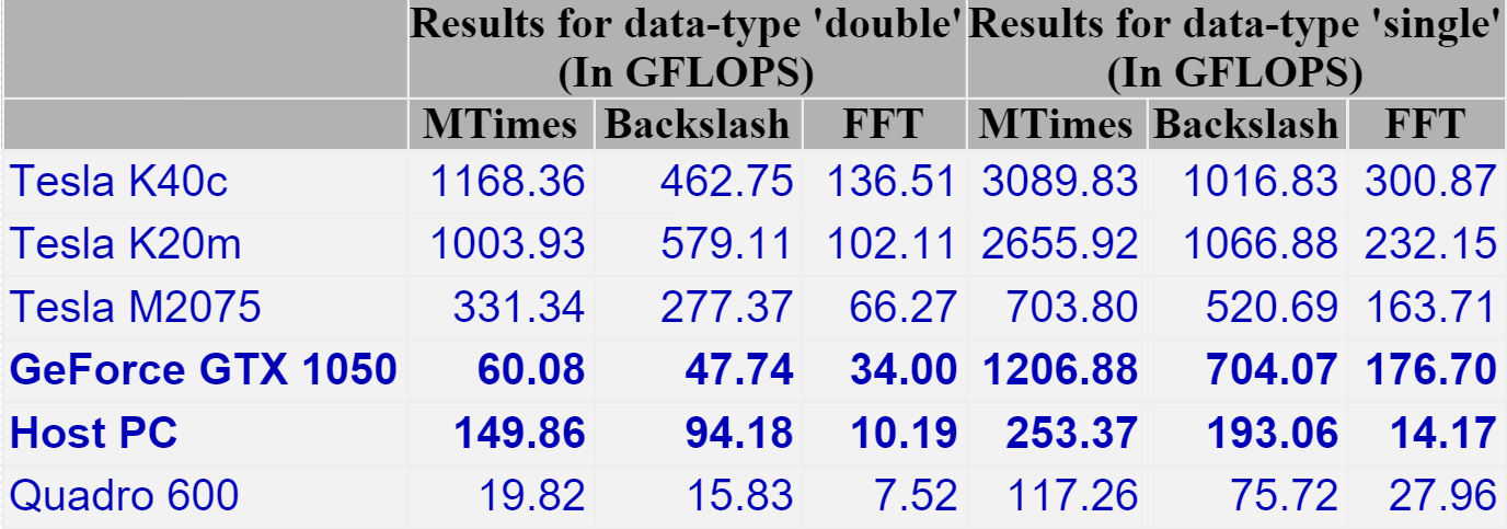
I last did this for my Retina MacBook Pro and am happy to see that the numbers are better across the board. The standout figure for me is the 1206 Gflops (That’s 1.2 Teraflops!) of single precision performance for Matrix-Matrix Multiply.
That figure of 1.2 Teraflops rang a bell for me and it took me a while to realise why…..
My laptop vs Manchester University’s old HPC system – Horace
Old timers like me (I’m almost 40) like to compare modern hardware with bygone supercomputers (1980s Crays vs mobile phones for example) and we know we are truly old when the numbers coming out of laptop benchmarks match the peak theoretical performance of institutional HPC systems we actually used as part of our career.
This has now finally happened to me! I was at the University of Manchester when it commissioned a HPC service called Horace and I was there when it was switched off in 2010 (only 6 and a bit years ago!). It was the University’s primary HPC service with a support team, helpdesk, sysadmins…the lot. The specs are still available on Manchester’s website:
- 24 nodes, each with 8 cores giving 192 cores in total.
- Each core had a theoretical peak compute performance of 6.4 double precision Gflop/s
- So a node had a theoretical peak performance of 51.2 Gflop/s
- The whole thing could theoretically manage 1.2 Teraflop/s
- It had four special ‘high memory’ nodes with 32Gb RAM each
Good luck getting that 1.2 Teraflops out of it in practice!
I get a big geek-kick out of the fact that my new laptop has the same amount of RAM as one of these ‘big memory’ nodes and that my laptop’s double precision CPU performance is on par with the combined power of 3 of Horace’s nodes. Furthermore, my laptop’s GPU can just about manage 1.2 Teraflop/s of single precision performance in MATLAB — on par with the total combined power of the HPC system*.
* (I know, I know….Horace’s numbers are for double precision and my GPU numbers are single precision — apples to oranges — but it still astonishes me that the headline numbers are the same — 1.2 Teraflops).
I work at The University of Sheffield where I am one of the leaders of the new Research Software Engineering function. One of the things that my group does is help people make use of Sheffield’s High Performance Computing cluster, Iceberg.
Iceberg is a heterogenous system with around 3440 CPU cores and a sprinkling of GPUs. It’s been in use for several years and has been upgraded a few times over that period. It’s a very traditional HPC system that makes use of Linux and a variant of Sun Grid Engine as the scheduler and had served us well.

A while ago, the sysadmin pointed me to a goldmine of a resource — Iceberg’s accounting log. This 15 Gigabyte file contains information on every job submitted since July 2009. That’s more than 7 years of the HPC usage of 3249 users — over 46 million individual jobs.
The file format is very straightforward. There’s one line per job and each line consists of a set of colon separated fields. The first few fields look like something like this:
long.q:node54.iceberg.shef.ac.uk:el:abc07de:
The username is field 4 and the number of slots used by the job is field 35. On our system, slots correspond to CPU cores. If you want to run a 16 core job, you ask for 16 slots.
With one line of awk, we can determine the maximum number of slots ever requested by each user.
gawk -F: '$35>=slots[$4] {slots[$4]=$35};END{for(n in slots){print n, slots[n]}}' accounting > ./users_max_slots.csv
As a quick check, I grepped the output file for my username and saw that the maximum number of cores I’d ever requested was 20. I ran a 32 core MPI ‘Hello World’ job, reran the line of awk and confirmed that my new maximum was 32 cores.
There are several ways I could have filtered the number of users but I was having awk lessons from David Jones so let’s create a new file containing the users who have only ever requested 1 slot.
gawk -F: '$35>=slots[$4] {slots[$4]=$35};END{for(n in slots){if(slots[n]==1){print n, slots[n]}}}' accounting > users_where_max_is_one_slot.csv
Running wc on these files allows us to determine how many users are in each group
wc users_max_slots.csv

3250  6498 32706 users_max_slots.csv
One of those users turned out to be a blank line so 3249 usernames have been used on Iceberg over the last 7 years.
wc users_where_max_is_one_slot.csv
2393  4786 23837 users_where_max_is_one_slot.csv
That is, 2393 of our 3249 users (just over 73%) over the last 7 years have only ever run 1 slot, and therefore 1 core, jobs.
High Performance?
So 73% of all users have only ever submitted single core jobs. This does not necessarily mean that they have not been making use of parallelism. For example, they might have been running job arrays – hundreds or thousands of single core jobs performing parameter sweeps or monte carlo simulations.
Maybe they were running parallel codes but only asked the scheduler for one core. In the early days this would have led to oversubscribed nodes, possibly up to 16 jobs, each trying to run 16 cores.These days, our sysadmin does some voodoo to ensure that jobs can only use the number of cores that have been requested, no matter how many threads their code is spawning. Either way, making this mistake is not great for performance.
Whatever is going on, this figure of 73% is surprising to me!
Thanks to David Jones for the awk lessons although if I’ve made a mistake, it’s all my fault!
Update (11th Jan 2017)
UCL’s Ian Kirker took a look at the usage of their general purpose cluster and found that 71.8% of their users have only ever run 1 core jobs. https://twitter.com/ikirker/status/819133966292807680
I was sat in a meeting recently where people were discussing High Performance Computing options. Someone had found some money down the back of the sofa and asked the rest of us how we’d spend it if it were ours (For the record, I wanted some big-memory nodes — 512Gb RAM minimum).
Halfway through the meeting someone asked about the parallel filesystem in use on Sheffield’s HPC systems and I answered Lustre — not expecting any further comment. I don’t know much about parallel I/O systems but I do know that all of the systems I have access to make use of Lustre. Sheffield’s Iceberg, Manchester’s Computational Shared Facility and the UK National supercomputer, Archer to name three. The Wikipedia page for Lustre suggests that it is very widely used in the HPC community worldwide.
I was surprised, then, when this comment was met with derision from some in the room. One person remarked ‘It’s a bit…um…classic..isn’t it?’, giving the impression that it was old and outdated. There was not much love for dear old Lustre it seemed!
There was no time in this meeting for me ask ‘What’s wrong with it then? Works fine for me!’so I did what I often do in times like this, I asked twitter:
Q for HPC followers. Is there anything wrong with using Lustre? Just been in a meeting where it was mocked as ‘classic’.
— Mike Croucher (@walkingrandomly) April 12, 2016
I found the responses to be very instructive so thought I would share them here. Here’s a comment from Ben Waugh
@walkingrandomly Lustre failures seem to be the main cause of downtime in my limited experience of large HPC systems.
— Ben Waugh (@benwaughuk) April 12, 2016
Not a great start! I’ve been hit by Lustre downtime too but, since I’m not a sysadmin, I haven’t got a genuine sense of how big a problem it is. It happens often enough that I’m aware of it but not so often that I feel the need to worry about it. Looking after large HPC systems is difficult and when one attempts to do do something difficult, the occasional failure is inevitable.
It seems that configuration might play a part in stability and performance. Peter Van Heusden kicked off with
@walkingrandomly Depending on the configuration can lack resilience, but is still standard HPC parallel FS.
— Peter van Heusden (@pvanheus) April 12, 2016
Adrian Jackson , Research Architect, HPC and Parallel Programmer, is thinking along similar lines.
@walkingrandomly 1/2 Yes, for a long time the metadata servers have not kept up, meaning you can destroy it with lots of small files
— Adrian Jackson (@adrianjhpc) April 12, 2016
@walkingrandomly 2/2 Although I believe this is being fixed in a variety of ways.
— Adrian Jackson (@adrianjhpc) April 12, 2016
@walkingrandomly Also, the default settings often don’t give best large scale performance, but that’s a matter of configuration
— Adrian Jackson (@adrianjhpc) April 12, 2016
Adrian also followed up with an interesting report on Performance of Parallel IO on ARCHER from June 2015. Thanks Adrian!
Glen K Lockwood is a Computational scientist specialising in I/O platforms at @NERSC, the flagship computing centre for the U.S. Dept. of Energy’s Office of Science. Glen has this insight,
@eoinbrazil @walkingrandomly Lustre just gets trashed because everyone uses it (because of its cost). Parallel file systems all misbehave
— Glenn K. Lockwood (@glennklockwood) April 12, 2016
I like this comment because it fits with my own, much less experienced, view of the parallel I/O world. A classic demonstration of confirmation bias perhaps but I see this thought pattern in a lot of areas. The pattern looks like this:
It’s hard to do ‘thing’. Most smart people do ‘thing’ with ‘foo’ and, since ‘thing’ is hard, many people have experienced problems with ‘foo’. Hence, people bash ‘foo’ a lot. ‘foo’ sucks!
Alternatives exist of course but there may be trade-offs. Here’s Mark Basham, software scientist @diamondlightsou in the UK.
@walkingrandomly we use it at Diamond for several of our file systems. GPFS is a bit better, but a lot more costly.
— Mark Basham (@basham_mark) April 12, 2016
I’ll give the final word to Nick Holway who sums up how I feel about parallel storage from a user’s point of view.
@walkingrandomly I like my HPC storage to be "classic" and also rather "boring"
— Nick Holway (@nickholway) April 12, 2016
Intel have finally released the Xeon Phi – an accelerator card based on 60 or so customised Intel cores to give around a Teraflop of double precision performance. That’s comparable to the latest cards from NVIDIA (1.3 Teraflops according to http://www.theregister.co.uk/2012/11/12/nvidia_tesla_k20_k20x_gpu_coprocessors/) but with one key difference—you don’t need to learn any new languages or technologies to take advantage of it (although you can do so if you wish)!
The Xeon Phi uses good, old fashioned High Performance Computing technologies that we’ve been using for years such as OpenMP and MPI. There’s no need to completely recode your algorithms in CUDA or OpenCL to get a performance boost…just a sprinkling of OpenMP pragmas might be enough in many cases. Obviously it will take quite a bit of work to squeeze every last drop of performance out of the thing but this might just be the realisation of ‘personal supercomputer’ we’ve all been waiting for.
Here are some links I’ve found so far — would love to see what everyone else has come up with. I’ll update as I find more
- http://www.theregister.co.uk/2012/11/12/intel_xeon_phi_coprocessor_launch/ (Includes pricing and some benchmarks)
- http://www.streamcomputing.eu/blog/2012-11-12/intels-answer-to-amd-and-nvidia-the-xeon-phi-5110p/ (lots of details, programming models and comparisons with GPUs)
- http://software.intel.com/en-us/blogs/2012/11/12/introducing-opencl-12-for-intel-xeon-phi-coprocessor (Intel’s OpenCL works on Xeon Phi)
- http://www.hpcwire.com/hpcwire/2012-11-12/nag_delivers_numerical_software_to_xeon_phi.html (My favourite numerical library has already been ported to the Phi)
I also note that the Xeon Phi uses AVX extensions but with a wider vector width of 512 bytes so if you’ve been taking advantage of that technology in your code (using one of these techniques perhaps) you’ll reap the benefits there too.
I, for one, am very excited and can’t wait to get my hands on one! Thoughts, comments and links gratefully received!
Updated 26th March 2015
I’ve been playing with AVX vectorisation on modern CPUs off and on for a while now and thought that I’d write up a little of what I’ve discovered. The basic idea of vectorisation is that each processor core in a modern CPU can operate on multiple values (i.e. a vector) simultaneously per instruction cycle.
Modern processors have 256bit wide vector units which means that each CORE can perform up to 16 double precision or 32 single precision floating point operations (FLOPS) per clock cycle. So, on a quad core CPU that’s typically found in a decent laptop you have 4 vector units (one per core) and could perform up to 64 double precision FLOPS per cycle. The Intel Xeon Phi accelerator unit has even wider vector units — 512bit!
This all sounds great but how does a programmer actually make use of this neat hardware trick? There are many routes:-
Intrinsics
At the ‘close to the metal’ level you code for these vector units using instructions called AVX intrinsics. This is relatively difficult and leads to none-portable code if you are not careful.
- The Intel Intrinsics Guide – An interactive reference tool for Intel intrinsic instructions,
- Introduction to Intel Advanced Vector Extensions – includes some example C++ programs using AVX intinsics
- Benefits of Intel AVX for small matrices – More code examples along with speed comparisons.
Auto-vectorisation in compilers
Since working with intrinsics is such hard work, why not let the compiler take the strain? Many modern compilers can automatically vectorize your C, C++ or Fortran code including gcc, PGI and Intel. Sometimes all you need to do is add an extra switch at compile time and reap the speed benefits. In truth, vectorization isn’t always automatic and the programmer needs to give the compiler some assistance but it is a lot easier than hand-coding intrinsics.
- A Guide to Auto-vectorization with Intel C++ Compilers – Exactly what it says. In my experience, the intel compilers do auto-vectorisation better than other compilers.
- Auto-vectorisation in gcc 4.7 – A superb article showing how auto-vectorisation works in practice when using gcc 4.7. Lots of C code examples along with the emitted assembler and a good discussion of the hints you may need to give to the compiler to get maximum performance.
- Auto-vectorisation in gcc – The project page for auto-vectorisation in gcc
- Optimizing Application Performance on x64 Processor-based Systems with PGI Compilers and Tools – Includes discussion and example of auto-vectorisation using the PGI compiler
- Jim Radigan: Inside Auto-Vectorization, 1 of n – A video by a Microsoft engineer working on Visual Studio 2012. A superb introduction to what vectorisation is along with speed-up demonstrations and discussion on how the auto-vectoriser will work in Visual Studio 2012.
- Auto Vectorizer in Visual Studio 2012 – A series of blog articles about vectorization in Visual Studio 2012.
Intel SPMD Program Compiler (ispc)
There is a midway point between automagic vectorisation and having to use intrinsics. Intel have a free compiler called ispc (http://ispc.github.com/) that allows you to write compute kernels in a modified subset of C. These kernels are then compiled to make use of vectorised instruction sets. Programming using ispc feels a little like using OpenCL or CUDA. I figured out how to hook it up to MATLAB a few months ago and developed a version of the Square Root function that is almost twice as fast as MATLAB’s own version for sandy bridge i7 processors.
- http://ispc.github.com/ – The website for ispc
- http://ispc.github.com/perf.html – Some performance metrics. In some cases combining vectorisation and parallelisation can increase single precision throughput by more than a factor of 32 on a quad-core machine!
- ispc: A SPMD Compiler For High-Performance CPU Programming, Illinois-Intel Parallelism Center Distinguished Speaker Series (UIUC), March 15, 2012. (talk video–requires Windows Media Player.) This link was taken from Matt Pharr’s website (The author of ispc).
OpenMP
OpenMP is an API specification for parallel programming that’s been supported by several compilers for many years. OpenMP 4 was released in mid 2013 and included support for vectorisation.
- Performance Essentials with OpenMP 4.0 Vectorization – A series of seven videos from Intel covering performance essentials using OpenMP 4.0 Vectorization with C/C++.
- Explicit Vector Programming with OpenMP 4.0 SIMD Extensions – A tutorial from HPC today.
Vectorised Libraries
Vendors of numerical libraries are steadily applying vectorisation techniques in order to maximise performance. If the execution speed of your application depends upon these library functions, you may get a significant speed boost simply by updating to the latest version of the library and recompiling with the relevant compiler flags.
- Yeppp! – A fast, vectorised math library (benchmarks here)
- NAG Library for Xeon Phi – A huge, commercial library for the Intel Xeon Phi Accelerator
- Intel AVX optimization in Intel Math Kernel Library (MKL) – See what’s been vectorised in version 10.3 of the MKL
- Intel Integrated Performance Primitives (IPP) Functions Optimized for AVX – The IPP library includes many basic algorithms used in image and signal processing
- SIMD Library for Evaluating Elementary Functions (SLEEF) – An open-source, vectorised library for the calculation of various mathematical functions. Someone has done benchmarks for it here.
- SIMD-oriented Fast Mersenne Twister (SFMT) – Uses vectorisation to implement a very fast random number generation.
CUDA for x86
Another route to vectorised code is to make use of the PGI Compiler’s support for x86 CUDA. What you do is take CUDA kernels written for NVIDIA GPUs and use the PGI Compiler to compile these kernels for x86 processors. The resulting executables take advantage of vectorisation. In essence, the vector units of the CPU are acting like CUDA cores–which they sort of are anyway!
The PGI compilers also have technology which they call PGI Unified binary which allows you to use NVIDIA GPUs when present or default to using multi-core x86 if no GPU is present.
- PGI CUDA-x86 – PGI’s main page for their CUDA on x86 technologies
OpenCL for x86 processors
Yet another route to vectorisation would be to use Intel’s OpenCL implementation which takes OpenCL kernels and compiles them down to take advantage of vector units (http://software.intel.com/en-us/blogs/2011/09/26/autovectorization-in-intel-opencl-sdk-15/). The AMD OpenCL implementation may also do this but I haven’t tried it and haven’t had chance to research it yet.
WalkingRandomly posts
I’ve written a couple of blog posts that made use of this technology.
- Using Intel’s SPMD Compiler (ispc) with MATLAB on Linux
- Using the Portland PGI Compiler for MATLAB mex files in Windows
Miscellaneous resources
There is other stuff out there but the above covers everything that I have used so far. I’ll finish by saying that everyone interested in vectorisation should check out this website…It’s the bible!
Research Articles on SSE/AVX vectorisation
I found the following research articles useful/interesting. I’ll add to this list over time as I dig out other articles.
Intel have just released their OpenCL Software Development Kit (SDK) for Intel processors. The good news is that this version targets the on-die GPU as well as the CPU allowing truly heterogeneous programming. The bad news is that the GPU goodness is for 3rd Generation ‘Ivy Bridge‘ Processors only– us backward Sandy Bridge users have been left in the cold :(
A quick scan through the release notes reveals the following:-
- OpenCL access to the on-die GPU part is currently for Windows only. Linux users only have CPU support at the moment.
- No access to the GPU part of Sandy Bridge Processors via this implementation.
- The GPU part has single precision only (I guess we’ll see many more mixed-precision algorithms from now on)
I don’t have access to an Ivy Bridge processor and so can’t have a play but I’m looking forward to seeing how much performance OpenCL programmers can squeeze out of this new implementation.
Other WalkingRandomly posts on GPU computing
Modern CPUs are capable of parallel processing at multiple levels with the most obvious being the fact that a typical CPU contains multiple processor cores. My laptop, for example, contains a quad-core Intel Sandy Bridge i7 processor and so has 4 processor cores. You may be forgiven for thinking that, with 4 cores, my laptop can do up to 4 things simultaneously but life isn’t quite that simple.
The first complication is hyper-threading where each physical core appears to the operating system as two or more virtual cores. For example, the processor in my laptop is capable of using hyper-threading and so I have access to up to 8 virtual cores! I have heard stories where unscrupulous sales people have passed off a 4 core CPU with hyperthreading as being as good as an 8 core CPU…. after all, if you fire up the Windows Task Manager you can see 8 cores and so there you have it! However, this is very far from the truth since what you really have is 4 real cores with 4 brain damaged cousins. Sometimes the brain damaged cousins can do something useful but they are no substitute for physical cores. There is a great explanation of this technology at makeuseof.com.
The second complication is the fact that each physical processor core contains a SIMD (Single Instruction Multiple Data) lane of a certain width. SIMD lanes, aka SIMD units or vector units, can process several numbers simultaneously with a single instruction rather than only one a time. The 256-bit wide SIMD lanes on my laptop’s processor, for example, can operate on up to 8 single (or 4 double) precision numbers per instruction. Since each physical core has its own SIMD lane this means that a 4 core processor could theoretically operate on up to 32 single precision (or 16 double precision) numbers per clock cycle!
So, all we need now is a way of programming for these SIMD lanes!
Intel’s SPMD Program Compiler, ispc, is a free product that allows programmers to take direct advantage of the SIMD lanes in modern CPUS using a C-like syntax. The speed-ups compared to single-threaded code can be impressive with Intel reporting up to 32 times speed-up (on an i7 quad-core) for a single precision Black-Scholes option pricing routine for example.
Using ispc on MATLAB
Since ispc routines are callable from C, it stands to reason that we’ll be able to call them from MATLAB using mex. To demonstrate this, I thought that I’d write a sqrt function that works faster than MATLAB’s built-in version. This is a tall order since the sqrt function is pretty fast and is already multi-threaded. Taking the square root of 200 million random numbers doesn’t take very long in MATLAB:
>> x=rand(1,200000000)*10;
>> tic;y=sqrt(x);toc
Elapsed time is 0.666847 seconds.
This might not be the most useful example in the world but I wanted to focus on how to get ispc to work from within MATLAB rather than worrying about the details of a more interesting example.
Step 1 – A reference single-threaded mex file
Before getting all fancy, let’s write a nice, straightforward single-threaded mex file in C and see how fast that goes.
#include <math.h>
#include "mex.h"

void mexFunction( int nlhs, mxArray *plhs[], int nrhs, const mxArray *prhs[] )
{
    double *in,*out;
    int rows,cols,num_elements,i;

    /*Get pointers to input matrix*/
    in = mxGetPr(prhs[0]);
    /*Get rows and columns of input matrix*/
    rows = mxGetM(prhs[0]);
    cols = mxGetN(prhs[0]);
    num_elements = rows*cols;

    /* Create output matrix */
    plhs[0] = mxCreateDoubleMatrix(rows, cols, mxREAL);
    /* Assign pointer to the output */
    out = mxGetPr(plhs[0]);

    for(i=0; i<num_elements; i++)
    {
        out[i] = sqrt(in[i]);
    }
}
Save the above to a text file called sqrt_mex.c and compile using the following command in MATLAB
mex sqrt_mex.c
Let’s check out its speed:
>> x=rand(1,200000000)*10;
>> tic;y=sqrt_mex(x);toc
Elapsed time is 1.993684 seconds.
Well, it works but it’s quite a but slower than the built-in MATLAB function so we still have some work to do.
Step 2 – Using the SIMD lane on one core via ispc
Using ispc is a two step process. First of all you need the .ispc program
export void ispc_sqrt(uniform double vin[], uniform double vout[],
                   uniform int count) {
    foreach (index = 0 ... count) {
        vout[index] = sqrt(vin[index]);
    }
}
Save this to a file called ispc_sqrt.ispc and compile it at the Bash prompt using
ispc -O2 ispc_sqrt.ispc -o ispc_sqrt.o -h ispc_sqrt.h --pic
This creates an object file, ispc_sqrt.o, and a header file, ispc_sqrt.h. Now create the mex file in MATLAB
#include <math.h>
#include "mex.h"
#include "ispc_sqrt.h"

void mexFunction( int nlhs, mxArray *plhs[], int nrhs, const mxArray *prhs[] )
{
    double *in,*out;
    int rows,cols,num_elements,i;

    /*Get pointers to input matrix*/
    in = mxGetPr(prhs[0]);
    /*Get rows and columns of input matrix*/
    rows = mxGetM(prhs[0]);
    cols = mxGetN(prhs[0]);
    num_elements = rows*cols;

    /* Create output matrix */
    plhs[0] = mxCreateDoubleMatrix(rows, cols, mxREAL);
    /* Assign pointer to the output */
    out = mxGetPr(plhs[0]);

    ispc::ispc_sqrt(in,out,num_elements);
}
Call this ispc_sqrt_mex.cpp and compile in MATLAB with the command
mex ispc_sqrt_mex.cpp ispc_sqrt.o
Let’s see how that does for speed:
>> tic;y=ispc_sqrt_mex(x);toc
Elapsed time is 1.379214 seconds.
So, we’ve improved on the single-threaded mex file a bit (1.37 instead of 2 seconds) but it’s still not enough to beat the MATLAB built-in. To do that, we are going to have to use the SIMD lanes on all 4 cores simultaneously.
Step 3 – A reference multi-threaded mex file using OpenMP
Let’s step away from ispc for a while and see how we do with something we’ve seen before– a mex file using OpenMP (see here and here for previous articles on this topic).
#include <math.h>
#include "mex.h"
#include <omp.h>

void do_calculation(double in[],double out[],int num_elements)
{
    int i;

#pragma omp parallel for shared(in,out,num_elements)
    for(i=0; i<num_elements; i++){
          out[i] = sqrt(in[i]);
         }
}

void mexFunction( int nlhs, mxArray *plhs[], int nrhs, const mxArray *prhs[] )
{
    double *in,*out;
    int rows,cols,num_elements,i;

    /*Get pointers to input matrix*/
    in = mxGetPr(prhs[0]);
    /*Get rows and columns of input matrix*/
    rows = mxGetM(prhs[0]);
    cols = mxGetN(prhs[0]);
    num_elements = rows*cols;

    /* Create output matrix */
    plhs[0] = mxCreateDoubleMatrix(rows, cols, mxREAL);
    /* Assign pointer to the output */
    out = mxGetPr(plhs[0]);

    do_calculation(in,out,num_elements);
}
Save this to a text file called openmp_sqrt_mex.c and compile in MATLAB by doing
mex openmp_sqrt_mex.c CFLAGS="\$CFLAGS -fopenmp" LDFLAGS="\$LDFLAGS -fopenmp"
Let’s see how that does (OMP_NUM_THREADS has been set to 4):
>> tic;y=openmp_sqrt_mex(x);toc
Elapsed time is 0.641203 seconds.
That’s very similar to the MATLAB built-in and I suspect that The Mathworks have implemented their sqrt function in a very similar manner. Theirs will have error checking, complex number handling and what-not but it probably comes down to a for-loop that’s been parallelized using Open-MP.
Step 4 – Using the SIMD lanes on all cores via ispc
To get a ispc program to run on all of my processors cores simultaneously, I need to break the calculation down into a series of tasks. The .ispc file is as follows
task void
ispc_sqrt_block(uniform double vin[], uniform double vout[],
                   uniform int block_size,uniform int num_elems){
    uniform int index_start = taskIndex * block_size;
    uniform int index_end = min((taskIndex+1) * block_size, (unsigned int)num_elems);

    foreach (yi = index_start ... index_end) {
        vout[yi] = sqrt(vin[yi]);
    }
}

export void
ispc_sqrt_task(uniform double vin[], uniform double vout[],
                   uniform int block_size,uniform int num_elems,uniform int num_tasks)
{

    launch[num_tasks] < ispc_sqrt_block(vin, vout, block_size, num_elems) >;
}
Compile this by doing the following at the Bash prompt
ispc -O2 ispc_sqrt_task.ispc -o ispc_sqrt_task.o -h ispc_sqrt_task.h --pic
We’ll need to make use of a task scheduling system. The ispc documentation suggests that you could use the scheduler in Intel’s Threading Building Blocks or Microsoft’s Concurrency Runtime but a basic scheduler is provided with ispc in the form of tasksys.cpp (I’ve also included it in the .tar.gz file in the downloads section at the end of this post), We’ll need to compile this too so do the following at the Bash prompt
g++ tasksys.cpp -O3 -Wall -m64 -c -o tasksys.o -fPIC
Finally, we write the mex file
#include <math.h>
#include "mex.h"
#include "ispc_sqrt_task.h"

void mexFunction( int nlhs, mxArray *plhs[], int nrhs, const mxArray *prhs[] )
{
    double *in,*out;
    int rows,cols,i;

    unsigned int num_elements;
    unsigned int block_size;
    unsigned int num_tasks;

    /*Get pointers to input matrix*/
    in = mxGetPr(prhs[0]);
    /*Get rows and columns of input matrix*/
    rows = mxGetM(prhs[0]);
    cols = mxGetN(prhs[0]);
    num_elements = rows*cols;

    /* Create output matrix */
    plhs[0] = mxCreateDoubleMatrix(rows, cols, mxREAL);
    /* Assign pointer to the output */
    out = mxGetPr(plhs[0]);

    block_size = 1000000;
    num_tasks = num_elements/block_size;

    ispc::ispc_sqrt_task(in,out,block_size,num_elements,num_tasks);

}
In the above, the input array is divided into tasks where each task takes care of 1 million elements. Our 200 million element test array will, therefore, be split into 200 tasks– many more than I have processor cores. I’ll let the task scheduler worry about how to schedule these tasks efficiently across the cores in my machine. Compile this in MATLAB by doing
mex ispc_sqrt_task_mex.cpp ispc_sqrt_task.o tasksys.o
Now for crunch time:
>> x=rand(1,200000000)*10;
>> tic;ys=sqrt(x);toc   %MATLAB's built-in
Elapsed time is 0.670766 seconds.
>> tic;y=ispc_sqrt_task_mex(x);toc  %my version using ispc
Elapsed time is 0.393870 seconds.
There we have it! A version of the sqrt function that works faster than MATLAB’s own by virtue of the fact that I am now making full use of the SIMD lanes in my laptop’s Sandy Bridge i7 processor thanks to ispc.
Although this example isn’t very useful as it stands, I hope that it shows that using the ispc compiler from within MATLAB isn’t as hard as you might think and is yet another tool in the arsenal of weaponry that can be used to make MATLAB faster.
Final Timings, downloads and links
- Single threaded: 2.01 seconds
- Single threaded with ispc: 1.37 seconds
- MATLAB built-in: 0.67 seconds
- Multi-threaded with OpenMP (OMP_NUM_THREADS=4): 0.64 seconds
- Multi-threaded with OpenMP and hyper-threading (OMP_NUM_THREADS=8): 0.55 seconds
- Task-based multicore with ispc: 0.39 seconds
Finally, here’s some links and downloads
System Specs
- MATLAB 2011b running on 64 bit linux
- gcc 4.6.1
- ispc version 1.1.1
- Intel Core i7-2630QM with 8Gb RAM
The NAG C Library is one of the largest commercial collections of numerical software currently available and I often find it very useful when writing MATLAB mex files. “Why is that?” I hear you ask.
One of the main reasons for writing a mex file is to gain more speed over native MATLAB. However, one of the main problems with writing mex files is that you have to do it in a low level language such as Fortran or C and so you lose much of the ease of use of MATLAB.
In particular, you lose straightforward access to most of the massive collections of MATLAB routines that you take for granted. Technically speaking that’s a lie because you could use the mex function mexCallMATLAB to call a MATLAB routine from within your mex file but then you’ll be paying a time overhead every time you go in and out of the mex interface. Since you are going down the mex route in order to gain speed, this doesn’t seem like the best idea in the world. This is also the reason why you’d use the NAG C Library and not the NAG Toolbox for MATLAB when writing mex functions.
One way out that I use often is to take advantage of the NAG C library and it turns out that it is extremely easy to add the NAG C library to your mex projects on Windows. Let’s look at a trivial example. The following code, nag_normcdf.c, uses the NAG function nag_cumul_normal to produce a simplified version of MATLAB’s normcdf function (laziness is all that prevented me from implementing a full replacement).
/* A simplified version of normcdf that uses the NAG C library
 * Written to demonstrate how to compile MATLAB mex files that use the NAG C Library
 * Only returns a normcdf where mu=0 and sigma=1
 * October 2011 Michael Croucher
 * www.walkingrandomly.com
 */

#include <math.h>
#include "mex.h"
#include "nag.h"
#include "nags.h"

void mexFunction( int nlhs, mxArray *plhs[], int nrhs, const mxArray *prhs[] )
{
    double *in,*out;
    int rows,cols,num_elements,i;

    if(nrhs>1)
    {
        mexErrMsgIdAndTxt("NAG:BadArgs","This simplified version of normcdf only takes 1 input argument");
    }

    /*Get pointers to input matrix*/
    in = mxGetPr(prhs[0]);
    /*Get rows and columns of input matrix*/
    rows = mxGetM(prhs[0]);
    cols = mxGetN(prhs[0]);
    num_elements = rows*cols;

    /* Create output matrix */
    plhs[0] = mxCreateDoubleMatrix(rows, cols, mxREAL);
    /* Assign pointer to the output */
    out = mxGetPr(plhs[0]);

    for(i=0; i<num_elements; i++){
          out[i] = nag_cumul_normal(in[i]);
         }
}
To compile this in MATLAB, just use the following command
mex nag_normcdf.c CLW6I09DA_nag.lib
If your system is set up the same as mine then the above should ‘just work’ (see System Information at the bottom of this post). The new function works just as you would expect it to
>> format long
>> format compact
>> nag_normcdf(1)
ans =
   0.841344746068543
Compare the result to normcdf from the statistics toolbox
>> normcdf(1)
ans =
   0.841344746068543
So far so good. I could stop the post here since all I really wanted to do was say ‘The NAG C library is useful for MATLAB mex functions and it’s a doddle to use – here’s a toy example and here’s the mex command to compile it’
However, out of curiosity, I looked to see if my toy version of normcdf was any faster than The Mathworks’ version. Let there be 10 million numbers:
>> x=rand(1,10000000);
Let’s time how long it takes MATLAB to take the normcdf of those numbers
>> tic;y=normcdf(x);toc
Elapsed time is 0.445883 seconds.
>> tic;y=normcdf(x);toc
Elapsed time is 0.405764 seconds.
>> tic;y=normcdf(x);toc
Elapsed time is 0.366708 seconds.
>> tic;y=normcdf(x);toc
Elapsed time is 0.409375 seconds.
Now let’s look at my toy-version that uses NAG.
>> tic;y=nag_normcdf(x);toc
Elapsed time is 0.544642 seconds.
>> tic;y=nag_normcdf(x);toc
Elapsed time is 0.556883 seconds.
>> tic;y=nag_normcdf(x);toc
Elapsed time is 0.553920 seconds.
>> tic;y=nag_normcdf(x);toc
Elapsed time is 0.540510 seconds.
So my version is slower! Never mind, I’ll just make my version parallel using OpenMP – Here is the code: nag_normcdf_openmp.c
/* A simplified version of normcdf that uses the NAG C library
 * Written to demonstrate how to compile MATLAB mex files that use the NAG C Library
 * Only returns a normcdf where mu=0 and sigma=1
 * October 2011 Michael Croucher
 * www.walkingrandomly.com
 */

#include <math.h>
#include "mex.h"
#include "nag.h"
#include "nags.h"
#include <omp.h>

void do_calculation(double in[],double out[],int num_elements)
{
    int i,tid;

#pragma omp parallel for shared(in,out,num_elements) private(i,tid)
    for(i=0; i<num_elements; i++){
          out[i] = nag_cumul_normal(in[i]);
         }
}

void mexFunction( int nlhs, mxArray *plhs[], int nrhs, const mxArray *prhs[] )
{
    double *in,*out;
    int rows,cols,num_elements;

    if(nrhs>1)
    {
        mexErrMsgIdAndTxt("NAG_NORMCDF:BadArgs","This simplified version of normcdf only takes 1 input argument");
    }

    /*Get pointers to input matrix*/
    in = mxGetPr(prhs[0]);
    /*Get rows and columns of input matrix*/
    rows = mxGetM(prhs[0]);
    cols = mxGetN(prhs[0]);
    num_elements = rows*cols;

    /* Create output matrix */
    plhs[0] = mxCreateDoubleMatrix(rows, cols, mxREAL);
    /* Assign pointer to the output */
    out = mxGetPr(plhs[0]);

    do_calculation(in,out,num_elements);
}
Compile that with
mex COMPFLAGS="$COMPFLAGS /openmp" nag_normcdf_openmp.c CLW6I09DA_nag.lib
and on my quad-core machine I get the following timings
>> tic;y=nag_normcdf_openmp(x);toc
Elapsed time is 0.237925 seconds.
>> tic;y=nag_normcdf_openmp(x);toc
Elapsed time is 0.197531 seconds.
>> tic;y=nag_normcdf_openmp(x);toc
Elapsed time is 0.206511 seconds.
>> tic;y=nag_normcdf_openmp(x);toc
Elapsed time is 0.211416 seconds.
This is faster than MATLAB and so normal service is resumed :)
System Information
- 64bit Windows 7
- MATLAB 2011b
- NAG C Library Mark 9 – CLW6I09DAL
- Visual Studio 2008
- Intel Core i7-2630QM processor