
Archive for May, 2010
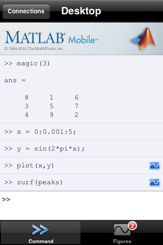
The Mathworks have released a new app for iPhone and iPad called MATLAB Mobile. When I first saw the headlines I was very excited but the product is rather disappointing in my opinion since all it does is offer a mobile interface to an instance of MATLAB running on a desktop machine. While this might be useful to some people I have to admit that it doesn’t light any fires for me. I’ll save my excitement for a mobile MATLAB application that can actually do some mathematics locally.
How about you though? Will this new application be useful for the way you work?
More articles from Walking Randomly on mobile mathematics software
Reading comma separated value (csv) files into MATLAB is trivial as long as the csv file you are trying to import is trivial. For example, say you wanted to import the file very_clean.txt which contains the following data
1031,-948,-76
507,635,-1148
-1031,948,750
-507,-635,114
The following, very simple command, is all that you need
>> veryclean = csvread('very_clean.txt')

veryclean =

        1031        -948         -76
         507         635       -1148
       -1031         948         750
        -507        -635         114
In the real world, however, your data is rarely this nice and clean. One of the most common problems faced by MATLABing data importers is that of header lines. Take the file quite_clean.txt for instance. This is identical to the previous example apart from the fact that it contains two header lines
These are some data that I made using my hand-crafted code
Date:12th July 1996
1031,-948,-76
507,635,-1148
-1031,948,750
-507,-635,114
This is all too much for the csvread command
>> data=csvread('quite_clean.txt')
??? Error using ==> dlmread at 145
Mismatch between file and format string.
Trouble reading number from file (row 1, field 1) ==> This

Error in ==> csvread at 52
    m=dlmread(filename, ',', r, c);
Not to worry, we can just use the more capable importdata command instead
>> quiteclean = importdata('quite_clean.txt')

quiteclean =

        data: [4x3 double]
    textdata: {2x1 cell}
The result above is a two element structure array and our numerical values are contained in a field called data. Here’s how you get at it.
>> quiteclean.data

ans =

        1031        -948         -76
         507         635       -1148
       -1031         948         750
        -507        -635         114
So far so good. How do we handle a file like messy_data.txt though?
header 1;
header 2;
1031,-948,-76, ,"12"
507,635,-1148, ,"34"
-1031,948,750, ,"45"
-507,-635,114, ,"67"
This is the kind of file encountered by Walking Randomly reader ‘reen’ and it contains exactly the same numerical values as the previous two examples. Unfortunately, it also contains some cruft that makes life more difficult for us. Let’s bring out the big-guns!
Using textscan to import csv files in MATLAB
When the going gets tough, the tough use textscan. Here’s the incantation for importing messy_data.txt
fid=fopen('messy_data.txt');
data = textscan(fid,'%f %f %f %*s %*s','HeaderLines',2,'Delimiter',',','CollectOutput',1);
fclose(fid)
The result is a one-element cell array that contains an array of doubles. Let’s get the array of doubles out of the cell
>> data=data{1}
data =
        1031        -948         -76
         507         635       -1148
       -1031         948         750
        -507        -635         114
If the importdata command is a chauffeur then textscan is a Ferrari and I don’t know about you but I’d much rather be driving my own Ferrari than being chauffeured around (John Cook over at The Endeavour has more to say on Ferraris and Chauffeurs).
Let’s de-construct the above set of commands. The first thing to notice is that, unlike csvread and importdata, you have to explicitly open and close your file when using the textscan command. So, you open your file using fopen and give it a file ID (which in this example is fid).
fid=fopen('messy_data.txt');
The first argument to textscan is just this file ID, fid. Next you need to supply a conversion specifier which in this case is
'%f %f %f %*s %*s'
The conversion specifier tells textscan what you want each row in your csv file to be converted to. %f means “64 bit double” and %s means “string” so ‘%f %f %f %s %s’ means “3 doubles followed by 2 strings” (we’ll get onto the asterisks in the original specifier later). You can use all sorts of data types in a conversion specifier such as integers, quoted strings and pattern matched strings among others. Check out the MATLAB documentation for textscan for the full list but an abbreviated list is shown below:
%d signed 32bit integer
%u unsigned 32bit integer
%f 64bit double (you'll want this most of the time when using MATLAB)
%s string
Now, in the command I used to import messy_data.txt the conversion specifier contained some asterisks such as %*s so what do these mean? Quite simply, the asterisk just means ‘ignore’ so %*s means ‘ignore the string in this field’. So, the full meaning of my conversion specifier ‘%f %f %f %*s %*s’ is “read 3 doubles and ignore 2 strings” and textscan will do this for every row.
The rest of the command is pretty self explanatory but I’ll explain it anyway for the sake of completeness
'HeaderLines',2
The file has 2 headerlines which should be ignored
'Delimiter',','
The fields are delimited (a posh word for separated) by a comma
'CollectOutput',1
If you supply a 1 (which stands for True) to the CollectOutput option then textscan will join consecutive output cells with the same data type into a single array. Since I want all of my doubles to be in a single array then this is the behaviour I went for.
Finally, once you have finished textscanning, don’t forget to close your file
fclose(fid)
That’s pretty much it for this mini-tutorial – I hope you find it useful.
Version 14 of Maple was released a couple of weeks ago and it appears to have some very cool stuff in it. Some of the highlights that stand out for me include
- Accelerated linear algebra using graphics cards via NVIDIA’s CUDA. Maple’s advertising blurb says that they have implemented matrix multiplication and that this will help speed up many linear algebra routines since this is such a fundamental operation. I think that Maple are the first of the big general purpose mathematical packages to offer direct CUDA integration out of the box and this development is well worth watching. The speed-ups that are possible from CUDA technology are nothing short of astonishing – hundreds of times in some cases. However, Maplesoft are going to need to add a lot more than matrix multiplication in order for this to be truly useful. A set of fast random number generators would be nice for example (I’m thinking superfast Monte-carlo simulations – the finance people would love it).
- Maple uses Intel’s Math Kernel Library (MKL) for many of its low-level numerical linear algebra routines and this has been updated to version 10.0 in Maple 14. For 32bit windows users this has sped certain operations up quite a lot but it is 64bit Windows users who will really see the benefit since 64bit Maple 13 only used a set of generic BLAS routines. The practical upshot is that certain basic linear algebra routines, such as Matrix Multiplication, can be around 10 times faster in 64bit windows Maple 14 compared to the previous version. I couldn’t find mention of the Linux version.
- A shed load of updates to their differential equation solvers including a new numerical routine called the Cash-Karp pair.
- The Maple toolbox for MATLAB is no longer a separate product and is now included with Maple itself. This is great news if you, like me, tend to work with several mathematical packages simultaneously. Of course you need to have a copy of MATLAB installed to make use of this functionality – you don’t get a copy of MATLAB for free :)
- You can now import MATLAB binary files (compressed and uncompressed) directly into Maple using the ImportMatrix command.
- Another product, The Maple-NAG connector, has also been integrated with Maple itself. This allows you to easily call the NAG C library directly from Maple but, similar to the MATLAB toolbox, you’ll have to purchase the NAG C library separately to make use of this.
As you can see, I tend to favour new features that lead to improved performance or better interoperability with other software packages in the first instance. New mathematics and usability features take a little longer to sink in (for me at least).
I’ve not got a copy of Maple 14 yet but will try to write more if I upgrade (finances permitting).
For a full list of changes check out Maple’s online help section.