
Archive for the ‘Making MATLAB faster’ Category
This article is the second part of a series where I look at rewriting a particular piece of MATLAB code using various techniques. The introduction to the series is here and the introduction to the larger series of GPU articles for MATLAB on WalkingRandomly is here.
Attempt 1 – Make as few modifications as possible
I took my best CPU-only code from last time (optimised_corr2.m) and changed a load of data-types from double to gpuArray in order to get the calculation to run on my laptop’s GPU using the parallel computing toolbox in MATLAB 2010b. I also switched to using the GPU versions of various functions such as parallel.gpu.GPUArray.randn instead of randn for example. Functions such as cumprod needed no modifications at all since they are nicely overloaded; if the argument to cumprod is of type double then the calculation happens on the CPU whereas if it is gpuArray then it happens on the GPU.
The above work took about a minute to do which isn’t bad for a CUDA ‘porting’ effort! The result, which I’ve called GPU_PCT_corr1.m is available for you to download and try out.
How about performance? Let’s do a quick tic and toc using my laptop’s NVIDIA GT 555M GPU.
>> tic;GPU_PCT_corr1;toc
Elapsed time is 950.573743 seconds.
The CPU version of this code took only 3.42 seconds which means that this GPU version is over 277 times slower! Something has gone horribly, horribly wrong!
Attempt 2 – Switch from script to function
In general functions should be faster than scripts in MATLAB because more automatic optimisations are performed on functions. I didn’t see any difference in the CPU version of this code (see optimised_corr3.m from part 1 for a CPU function version) and so left it as a script (partly so I had an excuse to discuss it here if I am honest). This GPU-version, however, benefits noticeably from conversion to a function. To do this, add the following line to the top of GPU_PCT_corr1.m
function [SimulPrices] = GPU_PTC_corr2( n,sub_size)
Next, you need to delete the following two lines
n=100000;                       %Number of simulations
sub_size = 125;
Finally, add the following to the end of our new function
end
That’s pretty much all I did to get GPU_PCT_corr2.m. Let’s see how that performs using the same parameters as our script (100,000 simulations in blocks of 125). I used script_vs_func.m to run both twice after a quick warm-up iteration and the results were:
Warm up
Elapsed time is 1.195806 seconds.
Main event
script
Elapsed time is 950.399920 seconds.
function
Elapsed time is 938.238956 seconds.
script
Elapsed time is 959.420186 seconds.
function
Elapsed time is 939.716443 seconds.
So, switching to a function has saved us a few seconds but performance is still very bad!
Attempt 3 – One big matrix multiply!
So far all I have done is take a program that works OK on a CPU, and run it exactly as-is on the GPU in the hope that something magical would happen to make it go faster. Of course, GPUs and CPUs are very different beasts with differing sets of strengths and weaknesses so it is rather naive to think that this might actually work. What we need to do is to play to the GPUs strengths more and the way to do this is to focus on this piece of code.
for i=1:sub_size
     CorrWiener(:,:,i)=parallel.gpu.GPUArray.randn(T-1,2)*UpperTriangle;
end
Here, we are performing lots of small matrix multiplications and, as mentioned in part 1, we might hope to get better performance by performing just one large matrix multiplication instead. To do this we can change the above code to
%Generate correlated random numbers
%using one big multiplication
randoms = parallel.gpu.GPUArray.randn(sub_size*(T-1),2);
CorrWiener = randoms*UpperTriangle;
CorrWiener = reshape(CorrWiener,(T-1),sub_size,2);
%CorrWiener = permute(CorrWiener,[1 3 2]); %Can't do this on the GPU in 2011b or below

%poor man's permute since GPU permute if not available in 2011b
CorrWiener_final = parallel.gpu.GPUArray.zeros(T-1,2,sub_size);
for s = 1:2
    CorrWiener_final(:, s, :) = CorrWiener(:, :, s);
end
The reshape and permute are necessary to get the matrix in the form needed later on. Sadly, MATLAB 2011b doesn’t support permute on GPUArrays and so I had to use the ‘poor mans permute’ instead.
The result of the above is contained in GPU_PCT_corr3.m so let’s see how that does in a fresh instance of MATLAB.
>> tic;GPU_PCT_corr3(100000,125);toc
Elapsed time is 16.666352 seconds.
>> tic;GPU_PCT_corr3(100000,125);toc
Elapsed time is 8.725997 seconds.
>> tic;GPU_PCT_corr3(100000,125);toc
Elapsed time is 8.778124 seconds.
The first thing to note is that performance is MUCH better so we appear to be on the right track. The next thing to note is that the first evaluation is much slower than all subsequent ones. This is totally expected and is due to various start-up overheads.
Recall that 125 in the above function calls refers to the block size of our monte-carlo simulation. We are doing 100,000 simulations in blocks of 125– a number chosen because I determined empirically that this was the best choice on my CPU. It turns out we are better off using much larger block sizes on the GPU:
>> tic;GPU_PCT_corr3(100000,250);toc
Elapsed time is 6.052939 seconds.
>> tic;GPU_PCT_corr3(100000,500);toc
Elapsed time is 4.916741 seconds.
>> tic;GPU_PCT_corr3(100000,1000);toc
Elapsed time is 4.404133 seconds.
>> tic;GPU_PCT_corr3(100000,2000);toc
Elapsed time is 4.223403 seconds.
>> tic;GPU_PCT_corr3(100000,5000);toc
Elapsed time is 4.069734 seconds.
>> tic;GPU_PCT_corr3(100000,10000);toc
Elapsed time is 4.039446 seconds.
>> tic;GPU_PCT_corr3(100000,20000);toc
Elapsed time is 4.068248 seconds.
>> tic;GPU_PCT_corr3(100000,25000);toc
Elapsed time is 4.099588 seconds.
The above, rather crude, test suggests that block sizes of 10,000 are the best choice on my laptop’s GPU. Sadly, however, it’s STILL slower than the 3.42 seconds I managed on the i7 CPU and represents the best I’ve managed using pure MATLAB code. The profiler tells me that the vast majority of the GPU execution time is spent in the cumprod line and in random number generation (over 40% each).
Trying a better GPU
Of course now that I have code that runs on a GPU I could just throw it at a better GPU and see how that does. I have access to MATLAB 2011b on a Tesla M2070 hooked up to a Linux machine so I ran the code on that. I tried various block sizes and the best time was 0.8489 seconds with the call GPU_PCT_corr3(100000,20000) which is just over 4 times faster than my laptop’s CPU.
Ask the Audience
Can you do better using just the GPU functionality provided in the Parallel Computing Toolbox (so no bespoke CUDA kernels or Jacket just yet)? I’ll be looking at how AccelerEyes’ Jacket myself in the next post.
Results so far
- Best CPU Result on laptop (i7-2630GM)with pure MATLAB code – 3.42 seconds
- Best GPU Result with PCT on laptop (GT555M) – 4.04 seconds
- Best GPU Result with PCT on Tesla M2070 – 0.85 seconds
Test System Specification
- Laptop model: Dell XPS L702X
- CPU: Intel Core i7-2630QM @2Ghz software overclockable to 2.9Ghz. 4 physical cores but total 8 virtual cores due to Hyperthreading.
- GPU: GeForce GT 555M with 144 CUDA Cores. Graphics clock: 590Mhz. Processor Clock:1180 Mhz. 3072 Mb DDR3 Memeory
- RAM: 8 Gb
- OS: Windows 7 Home Premium 64 bit.
- MATLAB: 2011b
Acknowledgements
Thanks to Yong Woong Lee of the Manchester Business School as well as various employees at The Mathworks for useful discussions and advice. Any mistakes that remain are all my own :)
Recently, I’ve been working with members of The Manchester Business School to help optimise their MATLAB code. We’ve had some great successes using techniques such as vectorisation, mex files and The NAG Toolbox for MATLAB (among others) combined with the raw computational power of Manchester’s Condor Pool (which I help run along with providing applications support).
A couple of months ago, I had the idea of taking a standard calculation in computational finance and seeing how fast I could make it run on MATLAB using various techniques. I’d then write these up and publish here for comment.
So, I asked one of my collaborators, Yong Woong Lee, a doctoral researcher in the Manchester Business School, if he could furnish me with a very simple piece computational finance code. I asked for something that was written to make it easy to see the underlying mathematics rather than for speed and he duly obliged with several great examples. I took one of these examples and stripped it down even further to its very bare bones. In doing so I may have made his example close to useless from a computational finance point of view but it gave me something nice and simple to play with.
What I ended up with was a simple piece of code that uses monte carlo techniques to find the distribution of two correlated assets: original_corr.m
%ORIGINAL_CORR - The original, unoptimised code that simulates two correlated assets
%% Correlated asset information
CurrentPrice = [78 102]; %Initial Prices of the two stocks
Corr = [1 0.4; 0.4 1]; %Correlation Matrix
T = 500; %Number of days to simulate = 2years = 500days
n = 100000; %Number of simulations
dt = 1/250; %Time step (1year = 250days)
Div=[0.01 0.01]; %Dividend
Vol=[0.2 0.3]; %Volatility
%%Market Information
r = 0.03; %Risk-free rate
%% Define storages
SimulPriceA=zeros(T,n); %Simulated Price of Asset A
SimulPriceA(1,:)=CurrentPrice(1);
SimulPriceB=zeros(T,n); %Simulated Price of Asset B
SimulPriceB(1,:)=CurrentPrice(2);
%% Generating the paths of stock prices by Geometric Brownian Motion
UpperTriangle=chol(Corr); %UpperTriangle Matrix by Cholesky decomposition
for i=1:n
Wiener=randn(T-1,2);
CorrWiener=Wiener*UpperTriangle;
for j=2:T
SimulPriceA(j,i)=SimulPriceA(j-1,i)*exp((r-Div(1)-Vol(1)^2/2)*dt+Vol(1)*sqrt(dt)*CorrWiener(j-1,1));
SimulPriceB(j,i)=SimulPriceB(j-1,i)*exp((r-Div(2)-Vol(2)^2/2)*dt+Vol(2)*sqrt(dt)*CorrWiener(j-1,2));
end
end
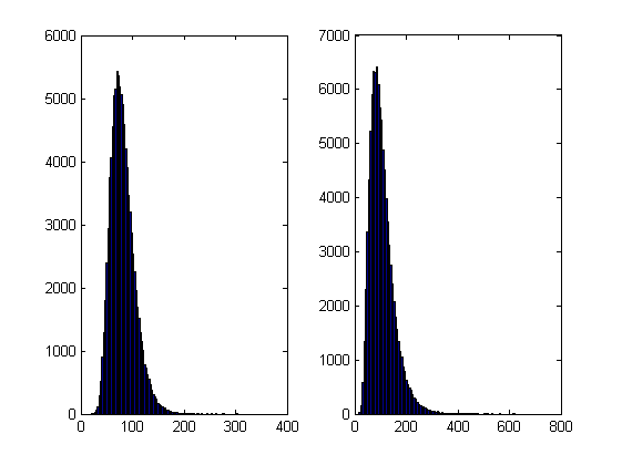
%% Plot the distribution of final prices
% Comment this section out if doing timings
% subplot(1,2,1);hist(SimulPriceA(end,:),100);
% subplot(1,2,2);hist(SimulPriceB(end,:),100);
On my laptop, this code takes 10.82 seconds to run on average. If you comment out the final two lines then it’ll take a little longer and will produce a histogram of the distribution of final prices.
I’m going to take this code and modify it in various ways to see how different techniques and technologies can make it run more quickly. Here is a list of everything I have done so far.
- Standard vectorisation (This article)
- Running on a GPU using the Parallel Computing Toolbox
- Running on a GPU using Jacket from AccelerEyes
Vectorisation – removing loops to make code go faster
Now, the most obvious optimisation that we can do with code like this is to use vectorisation to get rid of that double loop. The cumprod command is the key to doing this and the resulting code looks as follows: optimised_corr1.m
%OPTIMISED_CORR1 - A pure-MATLAB optimised code that simulates two correlated assets

%% Correlated asset information
CurrentPrice = [78 102];       %Initial Prices of the two stocks
Corr = [1 0.4; 0.4 1];         %Correlation Matrix
T = 500;                       %Number of days to simulate = 2years = 500days
Div=[0.01 0.01];               %Dividend
Vol=[0.2 0.3];                 %Volatility

%% Market Information
r = 0.03;                      %Risk-free rate

%% Simulation parameters
n=100000;                       %Number of simulation
dt=1/250;                       %Time step (1year = 250days)

%% Define storages
SimulPrices=repmat(CurrentPrice,n,1);
CorrWiener = zeros(T-1,2,n);

%% Generating the paths of stock prices by Geometric Brownian Motion
UpperTriangle=chol(Corr);    %UpperTriangle Matrix by Cholesky decomposition

for i=1:n
     CorrWiener(:,:,i)=randn(T-1,2)*UpperTriangle;
end
Volr = repmat(Vol,[T-1,1,n]);
Divr = repmat(Div,[T-1,1,n]);

%% do simulation
sim = cumprod(exp((r-Divr-Volr.^2./2).*dt+Volr.*sqrt(dt).*CorrWiener));
%get just the final prices
SimulPrices = SimulPrices.*reshape(sim(end,:,:),2,n)';

%% Plot the distribution of final prices
% Comment this section out if doing timings
%subplot(1,2,1);hist(SimulPrices(:,1),100);
%subplot(1,2,2);hist(SimulPrices(:,2),100);
This code takes an average of 4.19 seconds to run on my laptop giving us a factor of 2.58 times speed up over the original. This improvement in speed is not without its cost, however, and the price we have to pay is memory. Let’s take a look at the amount of memory used by MATLAB after running these two versions. First, the original
>> clear all
>> memory
Maximum possible array:              13344 MB (1.399e+010 bytes) *
Memory available for all arrays:     13344 MB (1.399e+010 bytes) *
Memory used by MATLAB:                 553 MB (5.800e+008 bytes)
Physical Memory (RAM):                8106 MB (8.500e+009 bytes)

*  Limited by System Memory (physical + swap file) available.
>> original_corr
>> memory
Maximum possible array:              12579 MB (1.319e+010 bytes) *
Memory available for all arrays:     12579 MB (1.319e+010 bytes) *
Memory used by MATLAB:                1315 MB (1.379e+009 bytes)
Physical Memory (RAM):                8106 MB (8.500e+009 bytes)

*  Limited by System Memory (physical + swap file) available.
Now for the vectorised version
>> %now I clear the workspace and check that all memory has been recovered%
>> clear all
>> memory
Maximum possible array:              13343 MB (1.399e+010 bytes) *
Memory available for all arrays:     13343 MB (1.399e+010 bytes) *
Memory used by MATLAB:                 555 MB (5.818e+008 bytes)
Physical Memory (RAM):                8106 MB (8.500e+009 bytes)

*  Limited by System Memory (physical + swap file) available.
>> optimised_corr1
>> memory
Maximum possible array:              10297 MB (1.080e+010 bytes) *
Memory available for all arrays:     10297 MB (1.080e+010 bytes) *
Memory used by MATLAB:                3596 MB (3.770e+009 bytes)
Physical Memory (RAM):                8106 MB (8.500e+009 bytes)

*  Limited by System Memory (physical + swap file) available.
So, the original version used around 762Mb of RAM whereas the vectorised version used 3041Mb. If you don’t have enough memory then you may find that the vectorised version runs very slowly indeed!
Adding a loop to the vectorised code to make it go even faster!
Simple vectorisation improvements such as the one above are sometimes so effective that it can lead MATLAB programmers to have a pathological fear of loops. This fear is becoming increasingly unjustified thanks to the steady improvements in MATLAB’s Just In Time (JIT) compiler. Discussing the details of MATLAB’s JIT is beyond the scope of these articles but the practical upshot is that you don’t need to be as frightened of loops as you used to.
In fact, it turns out that once you have finished vectorising your code, you may be able to make it go even faster by putting a loop back in (not necessarily thanks to the JIT though)! The following code takes an average of 3.42 seconds on my laptop bringing the total speed-up to a factor of 3.16 compared to the original. The only difference is that I have added a loop over the variable ii to split up the cumprod calculation over groups of 125 at a time.
I have a confession: I have no real idea why this modification causes the code to go noticeably faster. I do know that it uses a lot less memory; using the memory command, as I did above, I determined that it uses around 10Mb compared to 3041Mb of the original vectorised version. You may be wondering why I set sub_size to be 125 since I could have chosen any divisor of 100000. Well, I tried them all and it turned out that 125 was slightly faster than any other on my machine. Maybe we are seeing some sort of CPU cache effect? I just don’t know: optimised_corr2.m
%OPTIMISED_CORR2 - A pure-MATLAB optimised code that simulates two correlated assets
%% Correlated asset information
CurrentPrice = [78 102];       %Initial Prices of the two stocks
Corr = [1 0.4; 0.4 1];         %Correlation Matrix
T = 500;                       %Number of days to simulate = 2years = 500days
Div=[0.01 0.01];               %Dividend
Vol=[0.2 0.3];                 %Volatility

%% Market Information
r = 0.03;                      %Risk-free rate

%% Simulation parameters
n=100000;                       %Number of simulation
sub_size = 125;
dt=1/250;                       %Time step (1year = 250days)

%% Define storages
SimulPrices=repmat(CurrentPrice,n,1);
CorrWiener = zeros(T-1,2,sub_size);

%% Generating the paths of stock prices by Geometric Brownian Motion
UpperTriangle=chol(Corr);    %UpperTriangle Matrix by Cholesky decomposition
Volr = repmat(Vol,[T-1,1,sub_size]);
Divr = repmat(Div,[T-1,1,sub_size]);

for ii = 1:sub_size:n
   for i=1:sub_size
        CorrWiener(:,:,i)=randn(T-1,2)*UpperTriangle;
   end

   %% do simulation
   sim = cumprod(exp((r-Divr-Volr.^2./2).*dt+Volr.*sqrt(dt).*CorrWiener));
   %get just the final prices
   SimulPrices(ii:ii+sub_size-1,:) = SimulPrices(ii:ii+sub_size-1,:).*reshape(sim(end,:,:),2,sub_size)';
end
%% Plot the distribution of final prices
% Comment this section out if doing timings
%subplot(1,2,1);hist(SimulPrices(:,1),100);
%subplot(1,2,2);hist(SimulPrices(:,2),100);
Some things that might have worked (but didn’t)
- In general, functions are faster than scripts in MATLAB because MATLAB employs more aggressive optimisation techniques for functions. In this case, however, it didn’t make any noticeable difference on my machine. Try it out for yourself with optimised_corr3.m
- When generating the correlated random numbers, the above code performs lots of small matrix multiplications:
   for i=1:sub_size
        CorrWiener(:,:,i)=randn(T-1,2)*UpperTriangle;
   end
It is often the case that you can get more flops out of a system by doing a single large matrix-matrix multiply than lots of little ones. So, we could do this instead:
%Generate correlated random numbers
%using one big multiplication
randoms = randn(sub_size*(T-1),2);
CorrWiener = randoms*UpperTriangle;
CorrWiener = reshape(CorrWiener,(T-1),sub_size,2);
CorrWiener = permute(CorrWiener,[1 3 2]);
Sadly, however, any gains that we might have made by doing a single matrix-matrix multiply are lost when the resulting matrix is reshaped and permuted into the form needed for the rest of the code (on my machine at least). Feel free to try for yourself using optimised_corr4.m – the input argument of which determines the sub_size.
Ask the audience
Can you do better using nothing but pure matlab (i.e. no mex, parallel computing toolbox, GPUs or other such trickery…they are for later articles)? If so then feel free to contact me and let me know.
Acknowledgements
Thanks to Yong Woong Lee of the Manchester Business School as well as various employees at The Mathworks for useful discussions and advice. Any mistakes that remain are all my own :)
License
All code listed in this article is licensed under the 3-clause BSD license.
The test laptop
- Laptop model: Dell XPS L702X
- CPU: Intel Core i7-2630QM @2Ghz software overclockable to 2.9Ghz. 4 physical cores but total 8 virtual cores due to Hyperthreading.
- GPU: GeForce GT 555M with 144 CUDA Cores. Graphics clock: 590Mhz. Processor Clock:1180 Mhz. 3072 Mb DDR3 Memeory
- RAM: 8 Gb
- OS: Windows 7 Home Premium 64 bit.
- MATLAB: 2011b
Next Time
In the second part of this series I look at how to run this code on the GPU using The Mathworks’ Parallel Computing Toolbox.
Modern CPUs are capable of parallel processing at multiple levels with the most obvious being the fact that a typical CPU contains multiple processor cores. My laptop, for example, contains a quad-core Intel Sandy Bridge i7 processor and so has 4 processor cores. You may be forgiven for thinking that, with 4 cores, my laptop can do up to 4 things simultaneously but life isn’t quite that simple.
The first complication is hyper-threading where each physical core appears to the operating system as two or more virtual cores. For example, the processor in my laptop is capable of using hyper-threading and so I have access to up to 8 virtual cores! I have heard stories where unscrupulous sales people have passed off a 4 core CPU with hyperthreading as being as good as an 8 core CPU…. after all, if you fire up the Windows Task Manager you can see 8 cores and so there you have it! However, this is very far from the truth since what you really have is 4 real cores with 4 brain damaged cousins. Sometimes the brain damaged cousins can do something useful but they are no substitute for physical cores. There is a great explanation of this technology at makeuseof.com.
The second complication is the fact that each physical processor core contains a SIMD (Single Instruction Multiple Data) lane of a certain width. SIMD lanes, aka SIMD units or vector units, can process several numbers simultaneously with a single instruction rather than only one a time. The 256-bit wide SIMD lanes on my laptop’s processor, for example, can operate on up to 8 single (or 4 double) precision numbers per instruction. Since each physical core has its own SIMD lane this means that a 4 core processor could theoretically operate on up to 32 single precision (or 16 double precision) numbers per clock cycle!
So, all we need now is a way of programming for these SIMD lanes!
Intel’s SPMD Program Compiler, ispc, is a free product that allows programmers to take direct advantage of the SIMD lanes in modern CPUS using a C-like syntax. The speed-ups compared to single-threaded code can be impressive with Intel reporting up to 32 times speed-up (on an i7 quad-core) for a single precision Black-Scholes option pricing routine for example.
Using ispc on MATLAB
Since ispc routines are callable from C, it stands to reason that we’ll be able to call them from MATLAB using mex. To demonstrate this, I thought that I’d write a sqrt function that works faster than MATLAB’s built-in version. This is a tall order since the sqrt function is pretty fast and is already multi-threaded. Taking the square root of 200 million random numbers doesn’t take very long in MATLAB:
>> x=rand(1,200000000)*10;
>> tic;y=sqrt(x);toc
Elapsed time is 0.666847 seconds.
This might not be the most useful example in the world but I wanted to focus on how to get ispc to work from within MATLAB rather than worrying about the details of a more interesting example.
Step 1 – A reference single-threaded mex file
Before getting all fancy, let’s write a nice, straightforward single-threaded mex file in C and see how fast that goes.
#include <math.h>
#include "mex.h"

void mexFunction( int nlhs, mxArray *plhs[], int nrhs, const mxArray *prhs[] )
{
    double *in,*out;
    int rows,cols,num_elements,i;

    /*Get pointers to input matrix*/
    in = mxGetPr(prhs[0]);
    /*Get rows and columns of input matrix*/
    rows = mxGetM(prhs[0]);
    cols = mxGetN(prhs[0]);
    num_elements = rows*cols;

    /* Create output matrix */
    plhs[0] = mxCreateDoubleMatrix(rows, cols, mxREAL);
    /* Assign pointer to the output */
    out = mxGetPr(plhs[0]);

    for(i=0; i<num_elements; i++)
    {
        out[i] = sqrt(in[i]);
    }
}
Save the above to a text file called sqrt_mex.c and compile using the following command in MATLAB
mex sqrt_mex.c
Let’s check out its speed:
>> x=rand(1,200000000)*10;
>> tic;y=sqrt_mex(x);toc
Elapsed time is 1.993684 seconds.
Well, it works but it’s quite a but slower than the built-in MATLAB function so we still have some work to do.
Step 2 – Using the SIMD lane on one core via ispc
Using ispc is a two step process. First of all you need the .ispc program
export void ispc_sqrt(uniform double vin[], uniform double vout[],
                   uniform int count) {
    foreach (index = 0 ... count) {
        vout[index] = sqrt(vin[index]);
    }
}
Save this to a file called ispc_sqrt.ispc and compile it at the Bash prompt using
ispc -O2 ispc_sqrt.ispc -o ispc_sqrt.o -h ispc_sqrt.h --pic
This creates an object file, ispc_sqrt.o, and a header file, ispc_sqrt.h. Now create the mex file in MATLAB
#include <math.h>
#include "mex.h"
#include "ispc_sqrt.h"

void mexFunction( int nlhs, mxArray *plhs[], int nrhs, const mxArray *prhs[] )
{
    double *in,*out;
    int rows,cols,num_elements,i;

    /*Get pointers to input matrix*/
    in = mxGetPr(prhs[0]);
    /*Get rows and columns of input matrix*/
    rows = mxGetM(prhs[0]);
    cols = mxGetN(prhs[0]);
    num_elements = rows*cols;

    /* Create output matrix */
    plhs[0] = mxCreateDoubleMatrix(rows, cols, mxREAL);
    /* Assign pointer to the output */
    out = mxGetPr(plhs[0]);

    ispc::ispc_sqrt(in,out,num_elements);
}
Call this ispc_sqrt_mex.cpp and compile in MATLAB with the command
mex ispc_sqrt_mex.cpp ispc_sqrt.o
Let’s see how that does for speed:
>> tic;y=ispc_sqrt_mex(x);toc
Elapsed time is 1.379214 seconds.
So, we’ve improved on the single-threaded mex file a bit (1.37 instead of 2 seconds) but it’s still not enough to beat the MATLAB built-in. To do that, we are going to have to use the SIMD lanes on all 4 cores simultaneously.
Step 3 – A reference multi-threaded mex file using OpenMP
Let’s step away from ispc for a while and see how we do with something we’ve seen before– a mex file using OpenMP (see here and here for previous articles on this topic).
#include <math.h>
#include "mex.h"
#include <omp.h>

void do_calculation(double in[],double out[],int num_elements)
{
    int i;

#pragma omp parallel for shared(in,out,num_elements)
    for(i=0; i<num_elements; i++){
          out[i] = sqrt(in[i]);
         }
}

void mexFunction( int nlhs, mxArray *plhs[], int nrhs, const mxArray *prhs[] )
{
    double *in,*out;
    int rows,cols,num_elements,i;

    /*Get pointers to input matrix*/
    in = mxGetPr(prhs[0]);
    /*Get rows and columns of input matrix*/
    rows = mxGetM(prhs[0]);
    cols = mxGetN(prhs[0]);
    num_elements = rows*cols;

    /* Create output matrix */
    plhs[0] = mxCreateDoubleMatrix(rows, cols, mxREAL);
    /* Assign pointer to the output */
    out = mxGetPr(plhs[0]);

    do_calculation(in,out,num_elements);
}
Save this to a text file called openmp_sqrt_mex.c and compile in MATLAB by doing
mex openmp_sqrt_mex.c CFLAGS="\$CFLAGS -fopenmp" LDFLAGS="\$LDFLAGS -fopenmp"
Let’s see how that does (OMP_NUM_THREADS has been set to 4):
>> tic;y=openmp_sqrt_mex(x);toc
Elapsed time is 0.641203 seconds.
That’s very similar to the MATLAB built-in and I suspect that The Mathworks have implemented their sqrt function in a very similar manner. Theirs will have error checking, complex number handling and what-not but it probably comes down to a for-loop that’s been parallelized using Open-MP.
Step 4 – Using the SIMD lanes on all cores via ispc
To get a ispc program to run on all of my processors cores simultaneously, I need to break the calculation down into a series of tasks. The .ispc file is as follows
task void
ispc_sqrt_block(uniform double vin[], uniform double vout[],
                   uniform int block_size,uniform int num_elems){
    uniform int index_start = taskIndex * block_size;
    uniform int index_end = min((taskIndex+1) * block_size, (unsigned int)num_elems);

    foreach (yi = index_start ... index_end) {
        vout[yi] = sqrt(vin[yi]);
    }
}

export void
ispc_sqrt_task(uniform double vin[], uniform double vout[],
                   uniform int block_size,uniform int num_elems,uniform int num_tasks)
{

    launch[num_tasks] < ispc_sqrt_block(vin, vout, block_size, num_elems) >;
}
Compile this by doing the following at the Bash prompt
ispc -O2 ispc_sqrt_task.ispc -o ispc_sqrt_task.o -h ispc_sqrt_task.h --pic
We’ll need to make use of a task scheduling system. The ispc documentation suggests that you could use the scheduler in Intel’s Threading Building Blocks or Microsoft’s Concurrency Runtime but a basic scheduler is provided with ispc in the form of tasksys.cpp (I’ve also included it in the .tar.gz file in the downloads section at the end of this post), We’ll need to compile this too so do the following at the Bash prompt
g++ tasksys.cpp -O3 -Wall -m64 -c -o tasksys.o -fPIC
Finally, we write the mex file
#include <math.h>
#include "mex.h"
#include "ispc_sqrt_task.h"

void mexFunction( int nlhs, mxArray *plhs[], int nrhs, const mxArray *prhs[] )
{
    double *in,*out;
    int rows,cols,i;

    unsigned int num_elements;
    unsigned int block_size;
    unsigned int num_tasks;

    /*Get pointers to input matrix*/
    in = mxGetPr(prhs[0]);
    /*Get rows and columns of input matrix*/
    rows = mxGetM(prhs[0]);
    cols = mxGetN(prhs[0]);
    num_elements = rows*cols;

    /* Create output matrix */
    plhs[0] = mxCreateDoubleMatrix(rows, cols, mxREAL);
    /* Assign pointer to the output */
    out = mxGetPr(plhs[0]);

    block_size = 1000000;
    num_tasks = num_elements/block_size;

    ispc::ispc_sqrt_task(in,out,block_size,num_elements,num_tasks);

}
In the above, the input array is divided into tasks where each task takes care of 1 million elements. Our 200 million element test array will, therefore, be split into 200 tasks– many more than I have processor cores. I’ll let the task scheduler worry about how to schedule these tasks efficiently across the cores in my machine. Compile this in MATLAB by doing
mex ispc_sqrt_task_mex.cpp ispc_sqrt_task.o tasksys.o
Now for crunch time:
>> x=rand(1,200000000)*10;
>> tic;ys=sqrt(x);toc   %MATLAB's built-in
Elapsed time is 0.670766 seconds.
>> tic;y=ispc_sqrt_task_mex(x);toc  %my version using ispc
Elapsed time is 0.393870 seconds.
There we have it! A version of the sqrt function that works faster than MATLAB’s own by virtue of the fact that I am now making full use of the SIMD lanes in my laptop’s Sandy Bridge i7 processor thanks to ispc.
Although this example isn’t very useful as it stands, I hope that it shows that using the ispc compiler from within MATLAB isn’t as hard as you might think and is yet another tool in the arsenal of weaponry that can be used to make MATLAB faster.
Final Timings, downloads and links
- Single threaded: 2.01 seconds
- Single threaded with ispc: 1.37 seconds
- MATLAB built-in: 0.67 seconds
- Multi-threaded with OpenMP (OMP_NUM_THREADS=4): 0.64 seconds
- Multi-threaded with OpenMP and hyper-threading (OMP_NUM_THREADS=8): 0.55 seconds
- Task-based multicore with ispc: 0.39 seconds
Finally, here’s some links and downloads
System Specs
- MATLAB 2011b running on 64 bit linux
- gcc 4.6.1
- ispc version 1.1.1
- Intel Core i7-2630QM with 8Gb RAM
I recently spent a lot of time optimizing a MATLAB user’s code and made extensive use of mex files written in C. Now, one of the habits I have gotten into is to mix C and C++ style comments in my C source code like so:
/* This is a C style comment */

// This is a C++ style comment
For this particular project I did all of the development on Windows 7 using MATLAB 2011b and Visual Studio 2008 which had no problem with my mixing of comments. Move over to Linux, however, and it’s a very different story. When I try to compile my mex file
mex block1.c -largeArrayDims
I get the error message
block1.c:48: error: expected expression before ‘/’ token
The fix is to call mex as follows:
mex block1.c -largeArrayDims CFLAGS="\$CFLAGS -std=c99"
Hope this helps someone out there. For the record, I was using gcc and MATLAB 2011a on 64bit Scientific Linux.
The NAG C Library is one of the largest commercial collections of numerical software currently available and I often find it very useful when writing MATLAB mex files. “Why is that?” I hear you ask.
One of the main reasons for writing a mex file is to gain more speed over native MATLAB. However, one of the main problems with writing mex files is that you have to do it in a low level language such as Fortran or C and so you lose much of the ease of use of MATLAB.
In particular, you lose straightforward access to most of the massive collections of MATLAB routines that you take for granted. Technically speaking that’s a lie because you could use the mex function mexCallMATLAB to call a MATLAB routine from within your mex file but then you’ll be paying a time overhead every time you go in and out of the mex interface. Since you are going down the mex route in order to gain speed, this doesn’t seem like the best idea in the world. This is also the reason why you’d use the NAG C Library and not the NAG Toolbox for MATLAB when writing mex functions.
One way out that I use often is to take advantage of the NAG C library and it turns out that it is extremely easy to add the NAG C library to your mex projects on Windows. Let’s look at a trivial example. The following code, nag_normcdf.c, uses the NAG function nag_cumul_normal to produce a simplified version of MATLAB’s normcdf function (laziness is all that prevented me from implementing a full replacement).
/* A simplified version of normcdf that uses the NAG C library
 * Written to demonstrate how to compile MATLAB mex files that use the NAG C Library
 * Only returns a normcdf where mu=0 and sigma=1
 * October 2011 Michael Croucher
 * www.walkingrandomly.com
 */

#include <math.h>
#include "mex.h"
#include "nag.h"
#include "nags.h"

void mexFunction( int nlhs, mxArray *plhs[], int nrhs, const mxArray *prhs[] )
{
    double *in,*out;
    int rows,cols,num_elements,i;

    if(nrhs>1)
    {
        mexErrMsgIdAndTxt("NAG:BadArgs","This simplified version of normcdf only takes 1 input argument");
    }

    /*Get pointers to input matrix*/
    in = mxGetPr(prhs[0]);
    /*Get rows and columns of input matrix*/
    rows = mxGetM(prhs[0]);
    cols = mxGetN(prhs[0]);
    num_elements = rows*cols;

    /* Create output matrix */
    plhs[0] = mxCreateDoubleMatrix(rows, cols, mxREAL);
    /* Assign pointer to the output */
    out = mxGetPr(plhs[0]);

    for(i=0; i<num_elements; i++){
          out[i] = nag_cumul_normal(in[i]);
         }
}
To compile this in MATLAB, just use the following command
mex nag_normcdf.c CLW6I09DA_nag.lib
If your system is set up the same as mine then the above should ‘just work’ (see System Information at the bottom of this post). The new function works just as you would expect it to
>> format long
>> format compact
>> nag_normcdf(1)
ans =
   0.841344746068543
Compare the result to normcdf from the statistics toolbox
>> normcdf(1)
ans =
   0.841344746068543
So far so good. I could stop the post here since all I really wanted to do was say ‘The NAG C library is useful for MATLAB mex functions and it’s a doddle to use – here’s a toy example and here’s the mex command to compile it’
However, out of curiosity, I looked to see if my toy version of normcdf was any faster than The Mathworks’ version. Let there be 10 million numbers:
>> x=rand(1,10000000);
Let’s time how long it takes MATLAB to take the normcdf of those numbers
>> tic;y=normcdf(x);toc
Elapsed time is 0.445883 seconds.
>> tic;y=normcdf(x);toc
Elapsed time is 0.405764 seconds.
>> tic;y=normcdf(x);toc
Elapsed time is 0.366708 seconds.
>> tic;y=normcdf(x);toc
Elapsed time is 0.409375 seconds.
Now let’s look at my toy-version that uses NAG.
>> tic;y=nag_normcdf(x);toc
Elapsed time is 0.544642 seconds.
>> tic;y=nag_normcdf(x);toc
Elapsed time is 0.556883 seconds.
>> tic;y=nag_normcdf(x);toc
Elapsed time is 0.553920 seconds.
>> tic;y=nag_normcdf(x);toc
Elapsed time is 0.540510 seconds.
So my version is slower! Never mind, I’ll just make my version parallel using OpenMP – Here is the code: nag_normcdf_openmp.c
/* A simplified version of normcdf that uses the NAG C library
 * Written to demonstrate how to compile MATLAB mex files that use the NAG C Library
 * Only returns a normcdf where mu=0 and sigma=1
 * October 2011 Michael Croucher
 * www.walkingrandomly.com
 */

#include <math.h>
#include "mex.h"
#include "nag.h"
#include "nags.h"
#include <omp.h>

void do_calculation(double in[],double out[],int num_elements)
{
    int i,tid;

#pragma omp parallel for shared(in,out,num_elements) private(i,tid)
    for(i=0; i<num_elements; i++){
          out[i] = nag_cumul_normal(in[i]);
         }
}

void mexFunction( int nlhs, mxArray *plhs[], int nrhs, const mxArray *prhs[] )
{
    double *in,*out;
    int rows,cols,num_elements;

    if(nrhs>1)
    {
        mexErrMsgIdAndTxt("NAG_NORMCDF:BadArgs","This simplified version of normcdf only takes 1 input argument");
    }

    /*Get pointers to input matrix*/
    in = mxGetPr(prhs[0]);
    /*Get rows and columns of input matrix*/
    rows = mxGetM(prhs[0]);
    cols = mxGetN(prhs[0]);
    num_elements = rows*cols;

    /* Create output matrix */
    plhs[0] = mxCreateDoubleMatrix(rows, cols, mxREAL);
    /* Assign pointer to the output */
    out = mxGetPr(plhs[0]);

    do_calculation(in,out,num_elements);
}
Compile that with
mex COMPFLAGS="$COMPFLAGS /openmp" nag_normcdf_openmp.c CLW6I09DA_nag.lib
and on my quad-core machine I get the following timings
>> tic;y=nag_normcdf_openmp(x);toc
Elapsed time is 0.237925 seconds.
>> tic;y=nag_normcdf_openmp(x);toc
Elapsed time is 0.197531 seconds.
>> tic;y=nag_normcdf_openmp(x);toc
Elapsed time is 0.206511 seconds.
>> tic;y=nag_normcdf_openmp(x);toc
Elapsed time is 0.211416 seconds.
This is faster than MATLAB and so normal service is resumed :)
System Information
- 64bit Windows 7
- MATLAB 2011b
- NAG C Library Mark 9 – CLW6I09DAL
- Visual Studio 2008
- Intel Core i7-2630QM processor
So, you’re the proud owner of a new license for MATLAB’s parallel computing toolbox (PCT) and you are wondering how to get some bang for your buck as quickly as possible. Sure, you are going to learn about constructs such as parfor and spmd but that takes time and effort. Wouldn’t it be nice if you could speed up some of your MATLAB code simply by saying ‘Turn parallelisation on’?
It turns out that The Mathworks have been adding support for their parallel computing toolbox all over the place and all you have to do is switch it on (Assuming that you actually have the parallel computing toolbox of course). For example say you had the following call to fmincon (part of the optimisation toolbox) in your code
[x, fval] = fmincon(@objfun, x0, [], [], [], [], [], [], @confun,opts)
To turn on parallelisation across 2 cores just do
matlabpool 2;
opts = optimset('fmincon');
opts = optimset('UseParallel','always');
[x, fval] = fmincon(@objfun, x0, [], [], [], [], [], [], @confun,opts);
That wasn’t so hard was it? The speedup (if any) completely depends upon your particular optimization problem.
Why isn’t parallelisation turned on by default?
The next question that might occur to you is ‘Why doesn’t The Mathworks just turn parallelisation on by default?’ After all, although the above modification is straightforward, it does require you to know that this particular function supports parallel execution via the PCT. If you didn’t think to check then your code would be doomed to serial execution forever.
The simple answer to this question is ‘Sometimes the parallel version is slower‘. Take this serial code for example.
objfun = @(x)exp(x(1))*(4*x(1)^2+2*x(2)^2+4*x(1)*x(2)+2*x(2)+1);
confun = @(x) deal( [1.5+x(1)*x(2)-x(1)-x(2); -x(1)*x(2)-10], [] );
tic;
[x, fval] = fmincon(objfun, x0, [], [], [], [], [], [], confun);
toc
On the machine I am currently sat at (quad core running MATLAB 2011a on Linux) this typically takes around 0.032 seconds to solve. With a problem that trivial my gut feeling is that we are not going to get much out of switching to parallel mode.
objfun = @(x)exp(x(1))*(4*x(1)^2+2*x(2)^2+4*x(1)*x(2)+2*x(2)+1);
confun = @(x) deal( [1.5+x(1)*x(2)-x(1)-x(2); -x(1)*x(2)-10],[] );

%only do this next line once.  It opens two MATLAB workers
matlabpool 2;

opts = optimset('fmincon');
opts = optimset('UseParallel','always');

tic;
[x, fval] = fmincon(objfun, x0, [], [], [], [], [], [], confun,opts);
toc
Sure enough, this increases execution time dramatically to an average of 0.23 seconds on my machine. There is always a computational overhead that needs paying when you go parallel and if your problem is too trivial then this overhead costs more than the calculation itself.
So which functions support the Parallel Computing Toolbox?
I wanted a web-page that listed all functions that gain benefit from the Parallel Computing Toolbox but couldn’t find one. I found some documentation on specific toolboxes such as Parallel Statistics but nothing that covered all of MATLAB in one place. Here is my attempt at producing such a document. Feel free to contact me if I have missed anything out.
This covers MATLAB 2011b and is almost certainly incomplete. I’ve only covered toolboxes that I have access to and so some are missing. Please contact me if you have any extra information.
Bioinformatics Toolbox
Global Optimisation
- Various solvers use the PCT. See this part of the MATLAB documentation for details.
Image Processing
- blockproc
- Note that many Image Processing functions run in parallel even without the parallel computing toolbox. See my article Which MATLAB functions are Multicore Aware?
Optimisation Toolbox
Simulink
- Running parallel simulations
- You can increase the speed of diagram updates for models containing large model reference hierarchies by building referenced models that are configured in Accelerator mode in parallel whenever conditions allow. This is covered in the documentation.
Statistics Toolbox
- bootstrp
- bootci
- cordexch
- candexch
- crossval
- dcovary
- daugment
- growTrees
- jackknife
- lasso
- nnmf
- plsregress
- rowexch
- sequentialfs
- TreeBagger
Other articles about parallel computing in MATLAB from WalkingRandomly
- Which MATLAB functions are multicore aware? There are a ton of functions in MATLAB that take advantage of parallel processors automatically. No Parallel Computing Toolbox necessary.
- Parallel MATLAB with OpenMP mex files Want to parallelize your own functions without purchasing the PCT? Not afraid to get your hands dirty with C? Perhaps this option is for you.
- MATLAB GPU/CUDA Experiences and tutorials on my laptop – A series of articles where I look a GPU computing with CUDA on MATLAB
This is part 2 of an ongoing series of articles about MATLAB programming for GPUs using the Parallel Computing Toolbox. The introduction and index to the series is at https://www.walkingrandomly.com/?p=3730. All timings are performed on my laptop (hardware detailed at the end of this article) unless otherwise indicated.
Last time
In the previous article we saw that it is very easy to run MATLAB code on suitable GPUs using the parallel computing toolbox. We also saw that the GPU has its own area of memory that is completely separate from main memory. So, if you have a program that runs in main memory on the CPU and you want to accelerate part of it using the GPU then you’ll need to explicitly transfer data to the GPU and this takes time. If your GPU calculation is particularly simple then the transfer times can completely swamp your performance gains and you may as well not bother.
So, the moral of the story is either ‘Keep data transfers between GPU and host down to a minimum‘ or ‘If you are going to transfer a load of data to or from the GPU then make sure you’ve got a ton of work for the GPU to do.‘ Today, I’m going to consider the latter case.
A more complicated elementwise function – CPU version
Last time we looked at a very simple elementwise calculation– taking the sine of a large array of numbers. This time we are going to increase the complexity ever so slightly. Consider trig_series.m which is defined as follows
function out = myseries(t)
  out = 2*sin(t)-sin(2*t)+2/3*sin(3*t)-1/2*sin(4*t)+2/5*sin(5*t)-1/3*sin(6*t)+2/7*sin(7*t);
end
Let’s generate 75 million random numbers and see how long it takes to apply this function to all of them.
cpu_x = rand(1,75*1e6)*10*pi;
tic;myseries(cpu_x);toc
I did the above calculation 20 times using a for loop and took the median of the results to get 4.89 seconds1. Note that this calculation is fully parallelised…all 4 cores of my i7 CPU were working on the problem simultaneously (Many built in MATLAB functions are parallelised these days by the way…No extra toolbox necessary).
GPU version 1 (Or ‘How not to do it’)
One way of performing this calculation on the GPU would be to proceed as follows
cpu_x =rand(1,75*1e6)*10*pi;
tic
%Transfer data to GPU
gpu_x = gpuArray(cpu_x);
%Do calculation using GPU
gpu_y = myseries(gpu_x);
%Transfer results back to main memory
cpu_y = gather(gpu_y)
toc
The mean time of the above calculation on my laptop’s GPU is 3.27 seconds, faster than the CPU version but not by much. If you don’t include data transfer times in the calculation then you end up with 2.74 seconds which isn’t even a factor of 2 speed-up compared to the CPU.
GPU version 2 (arrayfun to the rescue)
We can get better performance out of the GPU simply by changing the line that does the calculation from
gpu_y = myseries(gpu_x);
to a version that uses MATLAB’s arrayfun command.
gpu_y = arrayfun(@myseries,gpu_x);
So, the full version of the code is now
cpu_x =rand(1,75*1e6)*10*pi;
tic
%Transfer data to GPU
gpu_x = gpuArray(cpu_x);
%Do calculation using GPU via arrayfun
gpu_y = arrayfun(@myseries,gpu_x);
%Transfer results back to main memory
cpu_y = gather(gpu_y)
toc
This improves the timings quite a bit. If we don’t include data transfer times then the arrayfun version completes in 1.42 seconds down from 2.74 seconds for the original GPU code. Including data transfer, the arrayfun version complete in 1.94 seconds compared to for the 3.27 seconds for the original.
Using arrayfun for the GPU is definitely the way to go! Giving the GPU every disadvantage I can think of (double precision, including transfer times, comparing against multi-thread CPU code etc) we still get a speed-up of just over 2.5 times on my laptop’s hardware. Pretty useful for hardware that was designed for energy-efficient gaming!
Note: Something that I learned while writing this post is that the first call to arrayfun will be slower than all of the rest. This is because arrayfun compiles the MATLAB function you pass it down to PTX and this can take a while (seconds). Subsequent calls will be much faster since arrayfun will use the compiled results. The compiled PTX functions are not saved between MATLAB sessions.
arrayfun – Good for your memory too!
Using the arrayfun function is not only good for performance, it’s also good for memory management. Imagine if I had 100 million elements to operate on instead of only 75 million. On my 3Gb GPU, the following code fails:
cpu_x = rand(1,100*1e6)*10*pi;
gpu_x = gpuArray(cpu_x);
gpu_y = myseries(gpu_x);
??? Error using ==> GPUArray.mtimes at 27
Out of memory on device. You requested: 762.94Mb, device has 724.21Mb free.

Error in ==> myseries at 3
        out =
        2*sin(t)-sin(2*t)+2/3*sin(3*t)-1/2*sin(4*t)+2/5*sin(5*t)-1/3*sin(6*t)+2/7*sin(7*t);
If we use arrayfun, however, then we are in clover. The following executes without complaint.
cpu_x = rand(1,100*1e6)*10*pi;
gpu_x = gpuArray(cpu_x);
gpu_y = arrayfun(@myseries,gpu_x);
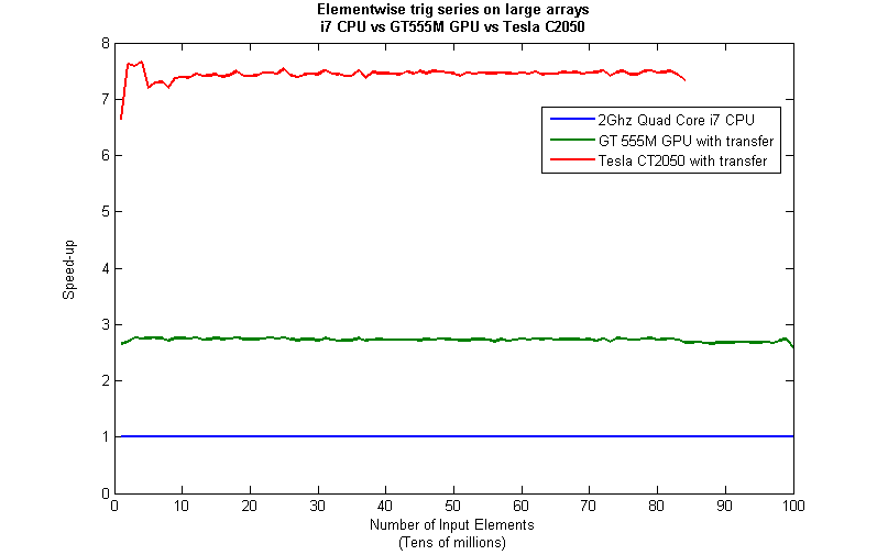
Some Graphs
Just like last time, I ran this calculation on a range of input arrays from 1 million to 100 million elements on both my laptop’s GT 555M GPU and a Tesla C2050 I have access to. Unfortunately, the C2050 is running MATLAB 2010b rather than 2011a so it’s not as fair a test as I’d like. I could only get up to 84 million elements on the Tesla before it exited due to memory issues. I’m not sure if this is down to the hardware itself or the fact that it was running an older version of MATLAB.

Next, I looked at the actual speed-up shown by the GPUs compared to my laptop’s i7 CPU. Again, this includes data transfer times, is in full double precision and the CPU version was multi-threaded (No dodgy ‘GPUs are awesome’ techniques used here). No matter what array size is used I get almost a factor of 3 speed-up using the laptop GPU and more than a factor of 7 speed-up when using the Tesla. Not too shabby considering that the programming effort to achieve this speed-up was minimal.
Conclusions
- It is VERY easy to modify simple, element-wise functions to take advantage of the GPU in MATLAB using the Parallel Computing Toolbox.
- arrayfun is the most efficient way of dealing with such functions.
- My laptop’s GPU demonstrated almost a 3 times speed-up compared to its CPU.
Hardware / Software used for the majority of this article
- Laptop model: Dell XPS L702X
- CPU: Intel Core i7-2630QM @2Ghz software overclockable to 2.9Ghz. 4 physical cores but total 8 virtual cores due to Hyperthreading.
- GPU: GeForce GT 555M with 144 CUDA Cores. Graphics clock: 590Mhz. Processor Clock:1180 Mhz. 3072 Mb DDR3 Memeory
- RAM: 8 Gb
- OS: Windows 7 Home Premium 64 bit. I’m not using Linux because of the lack of official support for Optimus.
- MATLAB: 2011a with the parallel computing toolbox
Code and sample timings (Will grow over time)
You need myseries.m and trigseries_test.m and the Parallel Computing Toolbox. These are the times given by the following function call for various systems (transfer included and using arrayfun).
[cpu,~,~,~,gpu] = trigseries_test(10,50*1e6,'mean')
GPUs
- Tesla C2050, Linux, 2010b – 0.4751 seconds
- NVIDIA GT 555M – 144 CUDA Cores, 3Gb RAM, Windows 7, 2011a – 1.2986 seconds
CPUs
- Intel Core i7-2630QM, Windows 7, 2011a (My laptop’s CPU) – 3.33 seconds
- Intel Core 2 Quad Q9650 @ 3.00GHz, Linux, 2011a – 3.9452 seconds
Footnotes
1 – This is the method used in all subsequent timings and is similar to that used by the File Exchange function, timeit (timeit takes a median, I took a mean). If you prefer to use timeit then the function call would be timeit(@()myseries(cpu_x)). I stick to tic and toc in the article because it makes it clear exactly where timing starts and stops using syntax well known to most MATLABers.
Thanks to various people at The Mathworks for some useful discussions, advice and tutorials while creating this series of articles.
This is part 1 of an ongoing series of articles about MATLAB programming for GPUs using the Parallel Computing Toolbox. The introduction and index to the series is at https://www.walkingrandomly.com/?p=3730.
Have you ever needed to take the sine of 100 million random numbers? Me either, but such an operation gives us an excuse to look at the basic concepts of GPU computing with MATLAB and get an idea of the timings we can expect for simple elementwise calculations.
Taking the sine of 100 million numbers on the CPU
Let’s forget about GPUs for a second and look at how this would be done on the CPU using MATLAB. First, I create 100 million random numbers over a range from 0 to 10*pi and store them in the variable cpu_x;
cpu_x = rand(1,100000000)*10*pi;
Now I take the sine of all 100 million elements of cpu_x using a single command.
cpu_y = sin(cpu_x)
I have to confess that I find the above command very cool. Not only are we looping over a massive array using just a single line of code but MATLAB will also be performing the operation in parallel. So, if you have a multicore machine (and pretty much everyone does these days) then the above command will make good use of many of those cores. Furthermore, this kind of parallelisation is built into the core of MATLAB….no parallel computing toolbox necessary. As an aside, if you’d like to see a list of functions that automatically run in parallel on the CPU then check out my blog post on the issue.
So, how quickly does my 4 core laptop get through this 100 million element array? We can find out using the MATLAB functions tic and toc. I ran it three times on my laptop and got the following
>> tic;cpu_y = sin(cpu_x);toc
Elapsed time is 0.833626 seconds.
>> tic;cpu_y = sin(cpu_x);toc
Elapsed time is 0.899769 seconds.
>> tic;cpu_y = sin(cpu_x);toc
Elapsed time is 0.916969 seconds.
So the first thing you’ll notice is that the timings vary and I’m not going to go into the reasons why here. What I am going to say is that because of this variation it makes sense to time the calculation a number of times (20 say) and take an average. Let’s do that
sintimes=zeros(1,20);
for i=1:20;tic;cpu_y = sin(cpu_x);sintimes(i)=toc;end
average_time = sum(sintimes)/20

average_time =
    0.8011
So, on average, it takes my quad core laptop just over 0.8 seconds to take the sine of 100 million elements using the CPU. A couple of points:
- I note that this time is smaller than any of the three test times I did before running the loop and I’m not really sure why. I’m guessing that it takes my CPU a short while to decide that it’s got a lot of work to do and ramp up to full speed but further insights are welcomed.
- While staring at the CPU monitor I noticed that the above calculation never used more than 50% of the available virtual cores. It’s using all 4 of my physical CPU cores but perhaps if it took advantage of hyperthreading I’d get even better performance? Changing OMP_NUM_THREADS to 8 before launching MATLAB did nothing to change this.
Taking the sine of 100 million numbers on the GPU
Just like before, we start off by using the CPU to generate the 100 million random numbers1
cpu_x = rand(1,100000000)*10*pi;
The first thing you need to know about GPUs is that they have their own memory that is completely separate from main memory. So, the GPU doesn’t know anything about the array created above. Before our GPU can get to work on our data we have to transfer it from main memory to GPU memory and we acheive this using the gpuArray command.
gpu_x = gpuArray(cpu_x); %this moves our data to the GPU
Once the GPU can see all our data we can apply the sine function to it very easily.
gpu_y = sin(gpu_x)
Finally, we transfer the results back to main memory.
cpu_y = gather(gpu_y)
If, like many of the GPU articles you see in the literature, you don’t want to include transfer times between GPU and host then you time the calculation like this:
tic
gpu_y = sin(gpu_x);
toc
Just like the CPU version, I repeated this calculation several times and took an average. The result was 0.3008 seconds giving a speedup of 2.75 times compared to the CPU version.
If, however, you include the time taken to transfer the input data to the GPU and the results back to the CPU then you need to time as follows
tic
gpu_x = gpuArray(cpu_x);
gpu_y = sin(gpu_x);
cpu_y = gather(gpu_y)
toc
On my system this takes 1.0159 seconds on average– longer than it takes to simply do the whole thing on the CPU. So, for this particular calculation, transfer times between host and GPU swamp the benefits gained by all of those CUDA cores.
Benchmark code
I took the ideas above and wrote a simple benchmark program called sine_test. The way you call it is as follows
[cpu,gpu_notransfer,gpu_withtransfer] = sin_test(numrepeats,num_elements]
For example, if you wanted to run the benchmarks 20 times on a 1 million element array and return the average times then you just do
>> [cpu,gpu_notransfer,gpu_withtransfer] = sine_test(20,1e6)
cpu =
    0.0085
gpu_notransfer =
    0.0022
gpu_withtransfer =
    0.0116
I then ran this on my laptop for array sizes ranging from 1 million to 100 million and used the results to plot the graph below.
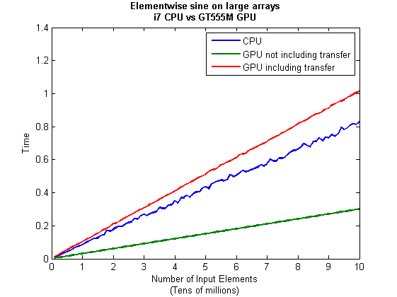
But I wanna write a ‘GPUs are awesome’ paper
So far in this little story things are not looking so hot for the GPU and yet all of the ‘GPUs are awesome’ papers you’ve ever read seem to disagree with me entirely. What on earth is going on? Well, lets take the advice given by csgillespie.wordpress.com and turn it on its head. How do we get awesome speedup figures from the above benchmarks to help us pump out a ‘GPUs are awesome paper’?
0. Don’t consider transfer times between CPU and GPU.
We’ve already seen that this can ruin performance so let’s not do it shall we? As long as we explicitly say that we are not including transfer times then we are covered.
1. Use a singlethreaded CPU.
Many papers in the literature compare the GPU version with a single-threaded CPU version and yet I’ve been using all 4 cores of my processor. Silly me…let’s fix that by running MATLAB in single threaded mode by launching it with the command
matlab -singleCompThread
Now when I run the benchmark for 100 million elements I get the following times
>> [cpu,gpu_no,gpu_with] = sine_test(10,1e8)
cpu =
    2.8875
gpu_no =
    0.3016
gpu_with =
    1.0205
Now we’re talking! I can now claim that my GPU version is over 9 times faster than the CPU version.
2. Use an old CPU.
My laptop has got one of those new-fangled sandy-bridge i7 processors…one of the best classes of CPU you can get for a laptop. If, however, I was doing these tests at work then I guess I’d be using a GPU mounted in my university Desktop machine. Obviously I would compare the GPU version of my program with the CPU in the Desktop….an Intel Core 2 Quad Q9650. Heck its running at 3Ghz which is more Ghz than my laptop so to the casual observer (or a phb) it would look like I was using a more beefed up processor in order to make my comparison fairer.
So, I ran the CPU benchmark on that (in singleCompThread mode obviously) and got 4.009 seconds…noticeably slower than my laptop. Awesome…I am definitely going to use that figure!
I know what you’re thinking…Mike’s being a fool for the sake of it but csgillespie.wordpress.com puts it like this ‘Since a GPU has (usually) been bought specifically for the purpose of the article, the CPU can be a few years older.’ So, some of those ‘GPU are awesome’ articles will be accidentally misleading us in exactly this manner.
3. Work in single precision.
Yeah I know that you like working with double precision arithmetic but that slows GPUs down. So, let’s switch to single precision. Just argue in your paper that single precision is OK for this particular calculation and we’ll be set. To change the benchmarking code all you need to do is change every instance of
rand(1,num_elems)*10*pi;
to
rand(1,num_elems,'single')*10*pi;
Since we are reputable researchers we will, of course, modify both the CPU and GPU versions to work in single precision. Timings are below
- Desktop at work (single thread, single precision): 3.49 seconds
- Laptop GPU (single precision, not including transfer): 0.122 seconds
OK, so switching to single precision made the CPU version a bit faster but it’s more than doubled GPU performance. We can now say that the GPU version is over 28 times faster than the CPU version. Now we have ourselves a bone-fide ‘GPUs are awesome’ paper.
4. Use the best GPU we can find
So far I have been comparing the CPU against the relatively lowly GPU in my laptop. Obviously, however, if I were to do this for real then I’d get a top of the range Tesla. It turns out that I know someone who has a Tesla C2050 and so we ran the single precision benchmark on that. The result was astonishing…0.0295 seconds for 100 million numbers not including transfer times. The double precision performance for the same calculation on the C2050 was 0.0524 seonds.
5. Write the abstract for our ‘GPUs are awesome’ paper
We took an Nvidia Tesla C2050 GPU and mounted it in a machine containing an Intel Quad Core CPU running at 3Ghz. We developed a program that performs element-wise trigonometry on arrays of up to 100 million single precision random numbers using both the CPU and the GPU. The GPU version of our code ran up to 118 times faster than the CPU version. GPUs are awesome!
Results from different CPUs and GPUs. Double precision, multi-threaded
I ran the sine_test benchmark on several different systems for 100 million elements. The CPU was set to be multi-threaded and double precision was used throughout.
sine_test(10,1e8)
GPUs
- Tesla C2050, Linux, 2011a – 0.7487 seconds including transfers, 0.0524 seconds excluding transfers.
- GT 555M – 144 CUDA Cores, 3Gb RAM, Windows 7, 2011a (My laptop’s GPU) -1.0205 seconds including transfers, 0.3016 seconds excluding transfers
CPUs
- Intel Core i7-880 @3.07Ghz, Linux, 2011a – 0.659 seconds
- Intel Core i7-2630QM, Windows 7, 2011a (My laptop’s CPU) – 0.801 seconds
- Intel Core 2 Quad Q9650 @ 3.00GHz, Linux – 0.958 seconds
Conclusions
- MATLAB’s new GPU functions are very easy to use! No need to learn low-level CUDA programming.
- It’s very easy to massage CPU vs GPU numbers to look impressive. Read those ‘GPUs are awesome’ papers with care!
- In real life you have to consider data transfer times between GPU and CPU since these can dominate overall wall clock time with simple calculations such as those considered here. The more work you can do on the GPU, the better.
- My laptop’s GPU is nowhere near as good as I would have liked it to be. Almost 6 times slower than a Tesla C2050 (excluding data transfer) for elementwise double precision calculations. Data transfer times seem to about the same though.
Next time
In the next article in the series I’ll look at an element-wise calculation that really is worth doing on the GPU – even using the wimpy GPU in my laptop – and introduce the MATLAB function arrayfun.
Footnote
1 – MATLAB 2011a can’t create random numbers directly on the GPU. I have no doubt that we’ll be able to do this in future versions of MATLAB which will change the nature of this particular calculation somewhat. Then it will make sense to include the random number generation in the overall benchmark; transfer times to the GPU will be non-existant. In general, however, we’ll still come across plenty of situations where we’ll have a huge array in main memory that needs to be transferred to the GPU for further processing so what we learn here will not be wasted.
Hardware / Software used for the majority of this article
- Laptop model: Dell XPS L702X
- CPU: Intel Core i7-2630QM @2Ghz software overclockable to 2.9Ghz. 4 physical cores but total 8 virtual cores due to Hyperthreading.
- GPU: GeForce GT 555M with 144 CUDA Cores. Graphics clock: 590Mhz. Processor Clock:1180 Mhz. 3072 Mb DDR3 Memeory
- RAM: 8 Gb
- OS: Windows 7 Home Premium 64 bit. I’m not using Linux because of the lack of official support for Optimus.
- MATLAB: 2011a with the parallel computing toolbox
Other GPU articles at Walking Randomly
- GPU Support in Mathematica, Maple, MATLAB and Maple Prime – See the various options available
- Insert new laptop to continue – My first attempt at using the GPU functionality in MATLAB
- NVIDIA lets down Linux laptop users – and how an open source project saves the day
Thanks to various people at The Mathworks for some useful discussions, advice and tutorials while creating this series of articles.
These days it seems that you can’t talk about scientific computing for more than 5 minutes without somone bringing up the topic of Graphics Processing Units (GPUs). Originally designed to make computer games look pretty, GPUs are massively parallel processors that promise to revolutionise the way we compute.
A brief glance at the specification of a typical laptop suggests why GPUs are the new hotness in numerical computing. Take my new one for instance, a Dell XPS L702X, which comes with a Quad-Core Intel i7 Sandybridge processor running at up to 2.9Ghz and an NVidia GT 555M with a whopping 144 CUDA cores. If you went back in time a few years and told a younger version of me that I’d soon own a 148 core laptop then young Mike would be stunned. He’d also be wondering ‘What’s the catch?’
Of course the main catch is that all processor cores are not created equally. Those 144 cores in my GPU are, individually, rather wimpy when compared to the ones in the Intel CPU. It’s the sheer quantity of them that makes the difference. The question at the forefront of my mind when I received my shiny new laptop was ‘Just how much of a difference?’
Now I’ve seen lots of articles that compare CPUs with GPUs and the GPUs always win…..by a lot! Dig down into the meat of these articles, however, and it turns out that things are not as simple as they seem. Roughly speaking, the abstract of some them could be summed up as ‘We took a serial algorithm written by a chimpanzee for an old, outdated CPU and spent 6 months parallelising and fine tuning it for a top of the line GPU. Our GPU version is up to 150 times faster!‘
Well it would be wouldn’t it?! In other news, Lewis Hamilton can drive his F1 supercar around Silverstone faster than my dad can in his clapped out 12 year old van! These articles are so prevalent that csgillespie.wordpress.com recently published an excellent article that summarised everything you should consider when evaluating them. What you do is take the claimed speed-up, apply a set of common sense questions and thus determine a realistic speedup. That factor of 150 can end up more like a factor of 8 once you think about it the right way.
That’s not to say that GPUs aren’t powerful or useful…it’s just that maybe they’ve been hyped up a bit too much!
So anyway, back to my laptop. It doesn’t have a top of the range GPU custom built for scientific computing, instead it has what Notebookcheck.net refers to as a fast middle class graphics card for laptops. It’s got all of the required bits though….144 cores and CUDA compute level 2.1 so surely it can whip the built in CPU even if it’s just by a little bit?
I decided to find out with a few randomly chosen tests. I wasn’t aiming for the kind of rigor that would lead to a peer reviewed journal but I did want to follow some basic rules at least
- I will only choose algorithms that have been optimised and parallelised for both the CPU and the GPU.
- I will release the source code of the tests so that they can be critised and repeated by others.
- I’ll do the whole thing in MATLAB using the new GPU functionality in the parallel computing toolbox. So, to repeat my calculations all you need to do is copy and paste some code. Using MATLAB also ensures that I’m using good quality code for both CPU and GPU.
The articles
This is the introduction to a set of articles about GPU computing on MATLAB using the parallel computing toolbox. Links to the rest of them are below and more will be added in the future.
- Elementwise operations on the GPU #1 – Basic commands using the PCT and how to write a ‘GPUs are awesome’ paper; no matter what results you get!
- Elementwise operations on the GPU #2 – A slightly more involved example showing a useful speed-up compared to the CPU. An introduction to MATLAB’s arrayfun
- Optimising a correlated asset calculation on MATLAB #1: Vectorisation on the CPU – A detailed look at a port from CPU MATLAB code to GPU MATLAB code.
- Optimising a correlated asset calculation on MATLAB #2: Using the GPU via the PCT – A detailed look at a port from CPU MATLAB code to GPU MATLAB code.
- Optimising a correlated asset calculation on MATLAB #3: Using the GPU via Jacket – A detailed look at a port from CPU MATLAB code to GPU MATLAB code.
External links of interest to MATLABers with an interest in GPUs
- The Parallel Computing Toolbox (PCT) – The Mathwork’s MATLAB add-on that gives you CUDA GPU support.
- Mike Gile’s MATLAB GPU Blog – from the University of Oxford
- Accelereyes – Developers of ‘Jacket’, an alternative to the parallel computing toolbox.
- A Mandelbrot Set on the GPU – Using the parallel computing toolbox to make pretty pictures…FAST!
- GP-you.org – A free CUDA-based GPU toolbox for MATLAB
- Matlab, CUDA and Me – Stu Blair gives various examples of calling CUDA kernels directly from MATLAB