
Optimising a correlated asset calculation on MATLAB #1 – Vectorisation on the CPU
Recently, I’ve been working with members of The Manchester Business School to help optimise their MATLAB code. We’ve had some great successes using techniques such as vectorisation, mex files and The NAG Toolbox for MATLAB (among others) combined with the raw computational power of Manchester’s Condor Pool (which I help run along with providing applications support).
A couple of months ago, I had the idea of taking a standard calculation in computational finance and seeing how fast I could make it run on MATLAB using various techniques. I’d then write these up and publish here for comment.
So, I asked one of my collaborators, Yong Woong Lee, a doctoral researcher in the Manchester Business School, if he could furnish me with a very simple piece computational finance code. I asked for something that was written to make it easy to see the underlying mathematics rather than for speed and he duly obliged with several great examples. I took one of these examples and stripped it down even further to its very bare bones. In doing so I may have made his example close to useless from a computational finance point of view but it gave me something nice and simple to play with.
What I ended up with was a simple piece of code that uses monte carlo techniques to find the distribution of two correlated assets: original_corr.m
%ORIGINAL_CORR - The original, unoptimised code that simulates two correlated assets
%% Correlated asset information
CurrentPrice = [78 102]; %Initial Prices of the two stocks
Corr = [1 0.4; 0.4 1]; %Correlation Matrix
T = 500; %Number of days to simulate = 2years = 500days
n = 100000; %Number of simulations
dt = 1/250; %Time step (1year = 250days)
Div=[0.01 0.01]; %Dividend
Vol=[0.2 0.3]; %Volatility
%%Market Information
r = 0.03; %Risk-free rate
%% Define storages
SimulPriceA=zeros(T,n); %Simulated Price of Asset A
SimulPriceA(1,:)=CurrentPrice(1);
SimulPriceB=zeros(T,n); %Simulated Price of Asset B
SimulPriceB(1,:)=CurrentPrice(2);
%% Generating the paths of stock prices by Geometric Brownian Motion
UpperTriangle=chol(Corr); %UpperTriangle Matrix by Cholesky decomposition
for i=1:n
Wiener=randn(T-1,2);
CorrWiener=Wiener*UpperTriangle;
for j=2:T
SimulPriceA(j,i)=SimulPriceA(j-1,i)*exp((r-Div(1)-Vol(1)^2/2)*dt+Vol(1)*sqrt(dt)*CorrWiener(j-1,1));
SimulPriceB(j,i)=SimulPriceB(j-1,i)*exp((r-Div(2)-Vol(2)^2/2)*dt+Vol(2)*sqrt(dt)*CorrWiener(j-1,2));
end
end
%% Plot the distribution of final prices
% Comment this section out if doing timings
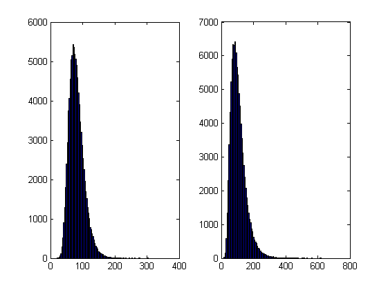
% subplot(1,2,1);hist(SimulPriceA(end,:),100);
% subplot(1,2,2);hist(SimulPriceB(end,:),100);
On my laptop, this code takes 10.82 seconds to run on average. If you comment out the final two lines then it’ll take a little longer and will produce a histogram of the distribution of final prices.
I’m going to take this code and modify it in various ways to see how different techniques and technologies can make it run more quickly. Here is a list of everything I have done so far.
- Standard vectorisation (This article)
- Running on a GPU using the Parallel Computing Toolbox
- Running on a GPU using Jacket from AccelerEyes
Vectorisation – removing loops to make code go faster
Now, the most obvious optimisation that we can do with code like this is to use vectorisation to get rid of that double loop. The cumprod command is the key to doing this and the resulting code looks as follows: optimised_corr1.m
%OPTIMISED_CORR1 - A pure-MATLAB optimised code that simulates two correlated assets

%% Correlated asset information
CurrentPrice = [78 102];       %Initial Prices of the two stocks
Corr = [1 0.4; 0.4 1];         %Correlation Matrix
T = 500;                       %Number of days to simulate = 2years = 500days
Div=[0.01 0.01];               %Dividend
Vol=[0.2 0.3];                 %Volatility

%% Market Information
r = 0.03;                      %Risk-free rate

%% Simulation parameters
n=100000;                       %Number of simulation
dt=1/250;                       %Time step (1year = 250days)

%% Define storages
SimulPrices=repmat(CurrentPrice,n,1);
CorrWiener = zeros(T-1,2,n);

%% Generating the paths of stock prices by Geometric Brownian Motion
UpperTriangle=chol(Corr);    %UpperTriangle Matrix by Cholesky decomposition

for i=1:n
     CorrWiener(:,:,i)=randn(T-1,2)*UpperTriangle;
end
Volr = repmat(Vol,[T-1,1,n]);
Divr = repmat(Div,[T-1,1,n]);

%% do simulation
sim = cumprod(exp((r-Divr-Volr.^2./2).*dt+Volr.*sqrt(dt).*CorrWiener));
%get just the final prices
SimulPrices = SimulPrices.*reshape(sim(end,:,:),2,n)';

%% Plot the distribution of final prices
% Comment this section out if doing timings
%subplot(1,2,1);hist(SimulPrices(:,1),100);
%subplot(1,2,2);hist(SimulPrices(:,2),100);
This code takes an average of 4.19 seconds to run on my laptop giving us a factor of 2.58 times speed up over the original. This improvement in speed is not without its cost, however, and the price we have to pay is memory. Let’s take a look at the amount of memory used by MATLAB after running these two versions. First, the original
>> clear all
>> memory
Maximum possible array:              13344 MB (1.399e+010 bytes) *
Memory available for all arrays:     13344 MB (1.399e+010 bytes) *
Memory used by MATLAB:                 553 MB (5.800e+008 bytes)
Physical Memory (RAM):                8106 MB (8.500e+009 bytes)

*  Limited by System Memory (physical + swap file) available.
>> original_corr
>> memory
Maximum possible array:              12579 MB (1.319e+010 bytes) *
Memory available for all arrays:     12579 MB (1.319e+010 bytes) *
Memory used by MATLAB:                1315 MB (1.379e+009 bytes)
Physical Memory (RAM):                8106 MB (8.500e+009 bytes)

*  Limited by System Memory (physical + swap file) available.
Now for the vectorised version
>> %now I clear the workspace and check that all memory has been recovered%
>> clear all
>> memory
Maximum possible array:              13343 MB (1.399e+010 bytes) *
Memory available for all arrays:     13343 MB (1.399e+010 bytes) *
Memory used by MATLAB:                 555 MB (5.818e+008 bytes)
Physical Memory (RAM):                8106 MB (8.500e+009 bytes)

*  Limited by System Memory (physical + swap file) available.
>> optimised_corr1
>> memory
Maximum possible array:              10297 MB (1.080e+010 bytes) *
Memory available for all arrays:     10297 MB (1.080e+010 bytes) *
Memory used by MATLAB:                3596 MB (3.770e+009 bytes)
Physical Memory (RAM):                8106 MB (8.500e+009 bytes)

*  Limited by System Memory (physical + swap file) available.
So, the original version used around 762Mb of RAM whereas the vectorised version used 3041Mb. If you don’t have enough memory then you may find that the vectorised version runs very slowly indeed!
Adding a loop to the vectorised code to make it go even faster!
Simple vectorisation improvements such as the one above are sometimes so effective that it can lead MATLAB programmers to have a pathological fear of loops. This fear is becoming increasingly unjustified thanks to the steady improvements in MATLAB’s Just In Time (JIT) compiler. Discussing the details of MATLAB’s JIT is beyond the scope of these articles but the practical upshot is that you don’t need to be as frightened of loops as you used to.
In fact, it turns out that once you have finished vectorising your code, you may be able to make it go even faster by putting a loop back in (not necessarily thanks to the JIT though)! The following code takes an average of 3.42 seconds on my laptop bringing the total speed-up to a factor of 3.16 compared to the original. The only difference is that I have added a loop over the variable ii to split up the cumprod calculation over groups of 125 at a time.
I have a confession: I have no real idea why this modification causes the code to go noticeably faster. I do know that it uses a lot less memory; using the memory command, as I did above, I determined that it uses around 10Mb compared to 3041Mb of the original vectorised version. You may be wondering why I set sub_size to be 125 since I could have chosen any divisor of 100000. Well, I tried them all and it turned out that 125 was slightly faster than any other on my machine. Maybe we are seeing some sort of CPU cache effect? I just don’t know: optimised_corr2.m
%OPTIMISED_CORR2 - A pure-MATLAB optimised code that simulates two correlated assets
%% Correlated asset information
CurrentPrice = [78 102];       %Initial Prices of the two stocks
Corr = [1 0.4; 0.4 1];         %Correlation Matrix
T = 500;                       %Number of days to simulate = 2years = 500days
Div=[0.01 0.01];               %Dividend
Vol=[0.2 0.3];                 %Volatility

%% Market Information
r = 0.03;                      %Risk-free rate

%% Simulation parameters
n=100000;                       %Number of simulation
sub_size = 125;
dt=1/250;                       %Time step (1year = 250days)

%% Define storages
SimulPrices=repmat(CurrentPrice,n,1);
CorrWiener = zeros(T-1,2,sub_size);

%% Generating the paths of stock prices by Geometric Brownian Motion
UpperTriangle=chol(Corr);    %UpperTriangle Matrix by Cholesky decomposition
Volr = repmat(Vol,[T-1,1,sub_size]);
Divr = repmat(Div,[T-1,1,sub_size]);

for ii = 1:sub_size:n
   for i=1:sub_size
        CorrWiener(:,:,i)=randn(T-1,2)*UpperTriangle;
   end

   %% do simulation
   sim = cumprod(exp((r-Divr-Volr.^2./2).*dt+Volr.*sqrt(dt).*CorrWiener));
   %get just the final prices
   SimulPrices(ii:ii+sub_size-1,:) = SimulPrices(ii:ii+sub_size-1,:).*reshape(sim(end,:,:),2,sub_size)';
end
%% Plot the distribution of final prices
% Comment this section out if doing timings
%subplot(1,2,1);hist(SimulPrices(:,1),100);
%subplot(1,2,2);hist(SimulPrices(:,2),100);
Some things that might have worked (but didn’t)
- In general, functions are faster than scripts in MATLAB because MATLAB employs more aggressive optimisation techniques for functions. In this case, however, it didn’t make any noticeable difference on my machine. Try it out for yourself with optimised_corr3.m
- When generating the correlated random numbers, the above code performs lots of small matrix multiplications:
   for i=1:sub_size
        CorrWiener(:,:,i)=randn(T-1,2)*UpperTriangle;
   end
It is often the case that you can get more flops out of a system by doing a single large matrix-matrix multiply than lots of little ones. So, we could do this instead:
%Generate correlated random numbers
%using one big multiplication
randoms = randn(sub_size*(T-1),2);
CorrWiener = randoms*UpperTriangle;
CorrWiener = reshape(CorrWiener,(T-1),sub_size,2);
CorrWiener = permute(CorrWiener,[1 3 2]);
Sadly, however, any gains that we might have made by doing a single matrix-matrix multiply are lost when the resulting matrix is reshaped and permuted into the form needed for the rest of the code (on my machine at least). Feel free to try for yourself using optimised_corr4.m – the input argument of which determines the sub_size.
Ask the audience
Can you do better using nothing but pure matlab (i.e. no mex, parallel computing toolbox, GPUs or other such trickery…they are for later articles)? If so then feel free to contact me and let me know.
Acknowledgements
Thanks to Yong Woong Lee of the Manchester Business School as well as various employees at The Mathworks for useful discussions and advice. Any mistakes that remain are all my own :)
License
All code listed in this article is licensed under the 3-clause BSD license.
The test laptop
- Laptop model: Dell XPS L702X
- CPU: Intel Core i7-2630QM @2Ghz software overclockable to 2.9Ghz. 4 physical cores but total 8 virtual cores due to Hyperthreading.
- GPU: GeForce GT 555M with 144 CUDA Cores. Graphics clock: 590Mhz. Processor Clock:1180 Mhz. 3072 Mb DDR3 Memeory
- RAM: 8 Gb
- OS: Windows 7 Home Premium 64 bit.
- MATLAB: 2011b
Next Time
In the second part of this series I look at how to run this code on the GPU using The Mathworks’ Parallel Computing Toolbox.
Hi!
You could use bsxfun to vectorize away all dimensions.
On my machine, this code ran a little fast than yours, over 80% of the time is actually used for random number generation.
UpperTriangle=chol(Corr); %UpperTriangle Matrix by Cholesky decomposition
randoms = reshape(randn(n*T,2)*UpperTriangle, [n, T, 2]);
Vol = permute(Vol,[3 1 2]);
Div = permute(Div,[3 1 2]);
SimulPriceAB = bsxfun(@times,cumprod(exp( bsxfun(@plus,(r-Div-Vol.^2/2)*dt,bsxfun(@times,Vol*sqrt(dt),randoms))),2),permute(CurrentPrice,[3 1 2]));
For fun, I tried the unoptimized code in Julia. See some discussion here: https://github.com/JuliaLang/julia/issues/445
Harald – thanks for that. I tried your version and it was indeed slightly faster (3.27 vs 3.42 seconds). However, it gave the wrong distribution. There is a possibility that my blog software has trashed your code. Feel free to email me the full thing and I’ll follow up.
Cheers,
Mike
@David – Julia looks VERY interesting. Love how easily you can switch BLAS versions! Thanks for that.