Walking Randomly

This article is the third part of a series where I look at rewriting a particular piece of MATLAB code using various techniques.  The introduction to the series is here and the introduction to the larger series of GPU articles for MATLAB is here.

Last time I used The Mathwork’s Parallel Computing Toolbox in order to modify a simple correlated asset calculation to run on my laptop’s GPU rather than its CPU.  Performance was not as good as I had hoped and I never managed to get my laptop’s GPU (an NVIDIA GT555M) to beat the CPU using functions from the parallel computing toolbox.  Transferring the code to a much more powerful Tesla GPU card resulted in a four times speed-up compared to the CPU in my laptop.

This time I’ll take a look at AccelerEyes’ Jacket, a third party GPU solution for MATLAB.

Attempt 1 – Make as few modifications as possible

I started off just as I did for the parallel computing toolbox GPU port; by taking the best CPU-only code from part 1 (optimised_corr2.m) and changing a load of data-types from double to gdouble in order to get the calculation to run on my laptop’s GPU using Jacket v1.8.1 and MATLAB 2010b.  I also switched to using the GPU versions of various functions such as grandn instead of randn for example.  Functions such as cumprod needed no  modifications at all since they are nicely overloaded; if the argument to cumprod is of type double then the calculation happens on the CPU whereas if it is gdouble then it happens on the GPU.

Now, one thing that I don’t like about Jacket’s implementation is that many of the functions return single precision numbers by default.  For example, if you do

a=grand(1,10)

then you end up with 10 numbers of type gsingle.  To get double precision numbers you have to do

grandn(1,10,'double')

Now you may be thinking ‘what’s the big deal? – it’s just a bit of syntax so get over it’ and I guess that would be a fair comment.  Supporting single precision also allows users of legacy GPUs to get in on the GPU-accelerated action which is a good thing. The problem as I see it is that almost everything else in MATLAB uses double precision numbers as the default and so it’s easy to get caught out.  I would much rather see functions such as grand return double precision by default with the option to use single precision if required–just like almost every other MATLAB function out there.

The result of my ‘port’ is GPU_jacket_corr1.m

One thing to note in this version, along with all subsequent Jacket versions, is the following command that appears at the very end of the program.

gsync;

This is very important if you want to get meaningful timing results since it ensures that all GPU computations have finished before execution continues. See the Jacket documentation on gysnc and this blog post on timing Jacket code for more details.

The other thing I’ll mention is that, in this version, I do this:

Corr = [1 0.4; 0.4 1];
UpperTriangle=gdouble(chol(Corr));

instead of

Corr = gdouble([1 0.4; 0.4 1]);
UpperTriangle=chol(Corr);

In other words, I do the cholesky decomposition on the CPU and move the results to the GPU rather than doing the calculation on the GPU.  This is mainly because I don’t have access to a Jacket DLA license but it’s probably the best thing to do anyway since such a small decomposition probably won’t happen any faster on the GPU.

So, how does it perform.  I ran it three times with the now usual parameters of 100000 simulations done in blocks of 125 (see the CPU version for how I came to choose 125)

>> tic;GPU_jacket_corr1;toc
Elapsed time is 40.691888 seconds.
>> tic;GPU_jacket_corr1;toc
Elapsed time is 32.096796 seconds.
>> tic;GPU_jacket_corr1;toc
Elapsed time is 32.039982 seconds.

Just like the Parallel Computing Toolbox, the first run is slower because of GPU warmup overheads. Also, just like the PCT, performance stinks! It’s clearly not enough, in this case at least, to blindly throw in a few gdoubles and hope for the best. It is worth noting, however, that this case is nowhere near as bad as the 900+ seconds we saw in the similar parallel computing toolbox version.

Jacket has punished me for being stupid (or optimistic if you want to be polite to me) but not as much as the PCT did.

Attempt 2 – Convert from a script to a function

When working with the Parallel Computing Toolbox I demonstrated that a switch from a script to a function yielded some speed-up.  This wasn’t the case with the Jacket version of the code.  The functional version, GPU_jacket_corr2.m, showed no discernable speed improvement compared to the script.

%Warm up run performed previously
>> tic;GPU_jacket_corr2(100000,125);toc
Elapsed time is 32.230638 seconds.
>> tic;GPU_jacket_corr2(100000,125);toc
Elapsed time is 32.179734 seconds.
>> tic;GPU_jacket_corr2(100000,125);toc
Elapsed time is 32.114864 seconds.

Attempt 3 – One big matrix multiply!

The original version of this calculation performs thousands of very small matrix multiplications and last time we saw that switching to a single, large matrix multiplication brought significant speed improvements on the GPU.  Modifying the code to do this with Jacket is a very similar process to doing it for the PCT so I’ll omit the details and just present the code, GPU_jacket_corr3.m

%Warm up runs performed previously
>> tic;GPU_jacket_corr3(100000,125);toc
Elapsed time is 2.041111 seconds.
>> tic;GPU_jacket_corr3(100000,125);toc
Elapsed time is 2.025450 seconds.
>> tic;GPU_jacket_corr3(100000,125);toc
Elapsed time is 2.032390 seconds.

Now that’s more like it! Finally we have a GPU version that runs faster than the CPU on my laptop. We can do better, however, since the block size of 125 was chosen especially for my CPU. With this Jacket version bigger is better and we get much more speed-up by switching to a block size of 25000 (I run out of memory on the GPU if I try even bigger block sizes).

%Warm up runs performed previously
>> tic;GPU_jacket_corr3(100000,25000);toc
Elapsed time is 0.749945 seconds.
>> tic;GPU_jacket_corr3(100000,25000);toc
Elapsed time is 0.749333 seconds.
>> tic;GPU_jacket_corr3(100000,25000);toc
Elapsed time is 0.749556 seconds.

Now this is exciting! My laptop GPU with Jacket 1.8.1 is faster than a high-end Tesla card using the parallel computing toolbox for this calculation. My excitement was short lived, however, when I looked at the resulting distribution. The random number generator in Jacket 1.8.1 gave a completely different distribution when compared to generators from other sources (I tried two CPU generators from The Mathworks and one from The Numerical Algorithms Group).  The only difference in the code that generated the results below is the random number generator used.

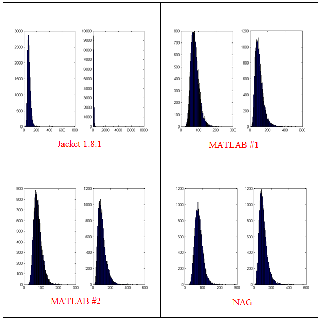
• The results shown in these plots were for only 20,000 simulations rather than the 100,000 I’ve been using elsewhere in this post. I found this bug in the development stage of these posts where I was using a smaller number of simulations.
• Jacket 1.8.1 is using Jackets old grandn function with the ‘double’ option set
• MATLAB #1 is using MATLAB’s randn using the Comb Recursive algorithm on the CPU
• MATLAB #2 is using MATLAB’s randn using the default Mersenne Twister on the CPU
• NAG is using a Wichman-Hill generator

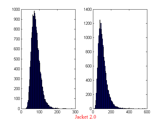
I sent my code to AccelerEye’s customer support who confirmed that this seemed to be a bug in their random number generator (an in-house Mersenne Twister implementation).  Less than a week later they offered me a new preview of Jacket from their Nightly builds where the old RNG had been replaced with the Mersenne Twister implementation produced by NVidia and I’m happy to confirm that not only does this fix the results for my code but it goes even faster!  Superb customer service!

This new RNG is now the default in version 2.0 of Jacket.  Here’s the distribution I get for 20,000 simulations (to stay in line with the plots shown above).

Switching back to 100,000 simulations to stay in line with all of the other benchmarks in this series gives the following times on my laptop’s GPU

%Warm up runs performed previously
>> tic;prices=GPU_jacket_corr3(100000,25000);toc
Elapsed time is 0.696891 seconds.
>> tic;prices=GPU_jacket_corr3(100000,25000);toc
Elapsed time is 0.697596 seconds.
>> tic;prices=GPU_jacket_corr3(100000,25000);toc
Elapsed time is 0.697312 seconds.

This is almost 5 times faster than the 3.42 seconds managed by the best CPU version from part 1. I sent my code to AccelerEyes and asked them to run it on a more powerful GPU, a Tesla C2075, and these are the results they sent back

Elapsed time is 5.246249 seconds. %warm up run
Elapsed time is 0.158165 seconds.
Elapsed time is 0.156529 seconds.
Elapsed time is 0.156522 seconds.
Elapsed time is 0.156501 seconds.

So, the Tesla is 4.45 times faster than my laptop’s GPU for this application and a very useful 21.85 times faster than my laptop’s CPU.

Results Summary

• Best CPU Result on laptop (i7-2630GM)with pure MATLAB code – 3.42 seconds
• Best GPU Result with PCT on laptop (GT555M) – 4.04 seconds
• Best GPU Result with PCT on Tesla M2070 – 0.85 seconds
• Best GPU Result with Jacket on laptop (GT555M) – 0.7 seconds
• Best GPU Result with Jacket on Tesla M2075 – 0.16 seconds

Test System Specification

• Laptop model: Dell XPS L702X
• CPU:Intel Core i7-2630QM @2Ghz software overclockable to 2.9Ghz. 4 physical cores but total 8 virtual cores due to Hyperthreading.
• GPU:GeForce GT 555M with 144 CUDA Cores.  Graphics clock: 590Mhz.  Processor Clock:1180 Mhz. 3072 Mb DDR3 Memeory
• RAM: 8 Gb
• OS: Windows 7 Home Premium 64 bit.
• MATLAB: 2011b

Acknowledgements

Thanks to Yong Woong Lee of the Manchester Business School as well as various employees at AccelerEyes for useful discussions and advice.  Any mistakes that remain are all my own.